This document discusses the derivation of backpropagation for neural networks. It begins with an overview of logistic regression and the sigmoid activation function. It then shows how to apply the chain rule to calculate the gradients needed for backpropagation. Specifically, it derives that the error term δ for each layer can be calculated as the error from the next layer multiplied by the weights and activation. This allows efficient computation of the gradient for each weight and bias term. Sample Python code is also provided to implement a basic neural network with backpropagation.

1. This draft was prepared using the LaTeX style file belonging to the Journal of Fluid Mechanics 1
Simple Backpropagation: Writing your own
Neural Network
Mohamamd Shafkat Amin1†
(Received xx; revised xx; accepted xx)
In this document, I discuss the derivation of back-propagation. First, I discuss the basics
of logistic regression and build on top of that and generalize for neural networks. I do
not talk about optimization algorithms [Sebastian (2016)] and only concentrate on the
basic mathematics behind backpropagation in this document. This document is meant
to be a first introduction to neural networks.
Key words: backpropagation, NN, logistic regression
1. Logistic Regression Primer
Before we discuss NNs, let’s start the discussion with logistic regression. In figure 2,
we have depicted the functions in logistic regression. Here Sigmoid function assumes the
following form:
Sigmoid(z) = σ(z) =
1
1 + e−z
and looks as shown in figure 1.
The loss function is:
L = −{
1
m m
(ylog (ˆy) + (1 − y) log (1 − ˆy))}
Here,
ˆy =
1
1 + e−z
z =
i
wixi + b
We will refer to ˆy as a (for activation for neural network) interchangeably.
We need to calculate derivatives:
∂L
∂wi
and
∂L
∂b
The reason why we compute gradient is because, negative gradient directs toward the
steepest descent along a function. As shown in figure 3, if we follow along the negative
gradient , we proceed toward the global minimum of a convex function. Discussion on
† Email address for correspondence: shafkat@gmail.com

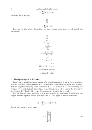
2. 2 Mohammad Shafkat Amin
[hc]
Figure 1. Sigmoid function [Source: Wikipedia]
Figure 2. Logistic Regression
Figure 3. Gradient descent[Library (2017)]
convexity of functions and local/global minima is beyond the scope of this document.
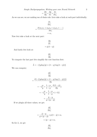
Let’s begin:
∂L
∂wi
=
∂L
∂z
∗
∂z
∂wi

3. Simple Backpropagation: Writing your own Neural Network 3
=
∂L
∂ˆy
∗
∂ˆy
∂z
∗
∂z
∂wi
As we can see, we are making use of chain rule. Lets take a look at each part individually:
∂z
∂wi
=
∂ (w1x1 + w2x2 + w3x3 + · · · )
∂wi
= wi
Now lets take a look at the next part:
∂ˆy
∂z
= ˆy (1 − ˆy)
And lastly lets look at:
∂L
∂ˆy
To compute the last part lets simplify the cost function first:
ˆL = −{(ylog (ˆy) + (1 − y) log (1 − ˆy))}
We can compute:
∂ ˆL
∂ˆy
=
∂ (−{(ylog (ˆy) + (1 − y) log (1 − ˆy))})
∂ˆy
= −{
y
ˆy
+
1 − y
1 − ˆy
∗
∂ (1 − ˆy)
∂ˆy
}
= −{
y
ˆy
+
1 − y
1 − ˆy
∗ (−1)}
=
ˆy − y
y ∗ (y − ˆy)
If we plugin all three values, we get:
∂ ˆL
∂wi
=
ˆy − y
y ∗ (y − ˆy)
∗ ˆy (1 − ˆy) ∗ wi
= (ˆy − y) ∗ wi
So for L, we get
∂L
∂wi

4. 4 Mohammad Shafkat Amin
= (ˆy − y) ∗ wi
Similarly for b, we get:
∂ ˆL
∂b
= (ˆy − y)
However, in the above discussion, we have glossed over how we calculated the
derivation:
∂ˆy
∂z
=
∂σ(z)
∂z
=
∂ 1
1+e−z
∂z
=
−(1 + e−z
)
(1 + e−z)2
=
e−z
(1 + e−z)2
=
1
(1 + e−z)
∗
e−z
(1 + e−z)
= σ(z) ∗ (1 − σ(z))
= ˆ(y) ∗ (1 − ˆ(y))
2. Backpropagation Primer
Let’s look at a arbitrary cross section of a neural network in figure 4. Let L represent
the last last layer in the network, L − 1 is the layer before that and so on and so forth.
Let the weights connecting nodes from layer L − i − 1 to layer L − i be denoted by the
weights WL−i and similarly the weights connecting layer L − 1 to layer L be denoted by
the weights WL. Let l ∈ {1, . . . , L} be an arbitrary layer in the network.
For the forward pass, lets look at how the weights, wi and biases bl influences the
ouput. Let the input to a node j in layer l be zl
j. This input is defined as follows:
zl
j =
i
wl
i,j ∗ al−1
i + bl
In matrix format, column vector:
zl
=





zl
1
z2
2
...
zl
j





(2.1)

5. Simple Backpropagation: Writing your own Neural Network 5
Figure 4. NN: Cross section
We then apply the activation function (sigmoid for the purpose of this document).
σ(zl
j) = al
j =
1
1 + e−zl
j
Rewriting the equation in matrix format, we get input to layer l
zl
= (wl
)T
∗ al−1
+ bl
And activation for layer l:
al
= σ(zl
)
In matrix format, al
vector looks like following:
al
=





σ(zl
1)
σ(z2
2)
...
σ(zl
j)





(2.2)
Regular Format Matrix Format
zl
j = i wl
i,j ∗ al−1
i + bl
zl
= (wl
)T
∗ al−1
+ bl
al
i = σ(zl
i) al
= σ(zl
)
Lets look at the simple cost function that we will be using for the scope of this document:
C =
1
2
(yL
i − aL
i )2

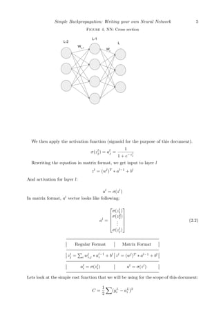
6. 6 Mohammad Shafkat Amin
To learn more about different cost functions see [Christopher (2016)] Here aL
i is the
output of the activation function from the last layer. We need to calculate the partial
derivative with respect to the parameters. For the last layer lets assume the following
notations:
∂C
∂zL
j
= δL
j
And for any arbitrary layer l, we have:
∂C
∂zl
j
= δl
j
In essence, backpropagation facilitates efficient computation of a massive chain rule
problem. To efficiently apply chain rule, in backpropagation, we compute and store δl
j
values and reuse them instead of recomputing redundantly. Let’s expand on the last layer:
∂C
∂zL
j
=
∂C
∂aL
j
∗
∂aL
j
∂zL
j
= (aL
j − yL
j ) ∗
∂σ(zL
j )
∂zL
j
= (aL
j − yL
j ) ∗ σ (zL
j )
Hence, we have calculated:
δL
j = (aL
j − yL
j ) ∗ σ (zL
j )
The first part of the equation is derived from following:
∂C
∂aL
j
=
∂ 1
2 (yL
i − aL
i )2
∂aL
j
=
∂ 1
2 {(yL
1 − aL
1 )2
+ . . . + (yL
2 − aL
2 )2
+ (yL
j − aL
j )2
+ . . .}
∂aL
j
= (aL
j − yL
j )
Now let’s generalize the computation for any arbitrary layer l. We want to compute:
δl
i =
∂C
∂zl
i
If we change the value of zl
i (red node in figure 5),the change propagates to many nodes
in the following layer (red edges in the figure).
δl
i =
∂C
∂zl
i
=
k
∂C
∂zl+1
k
∗
∂zl+1
k
∂zl
i

7. Simple Backpropagation: Writing your own Neural Network 7
Figure 5. NN: Backpropagation
=
k
δl+1
k ∗
∂zl+1
k
∂zl
i
=
k
δl+1
k ∗
∂(wl+1
1,k σ(zl
1) + wl+1
2,k σ(zl
2) + . . . + wl+1
i,k σ(zl
i) + . . .)
∂zl
i
=
k
δl+1
k ∗ wl+1
i,k ∗ σ (zl
i)
=
k
wl+1
i,k ∗ δl+1
k ∗ σ (zl
i)
In matrix form we get:
= wl+1
∗ δl+1
σ (zl
)
Here represents the hadamard product. To see how we have derived the above
equation, lets revisit what zl
j stands for
zl
j =
i
wl
i,j ∗ al
i + bl
Lets rewrite it for layer l + 1 and node k:
zl+1
k =
i
wl+1
i,k ∗ al
i + bl+1
Hence:
∂zl+1
k
∂zl
i

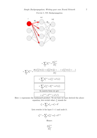
8. 8 Mohammad Shafkat Amin
=
∂(wl+1
i,k ∗ al
i)
∂zl
i
= wl+1
i,k ∗ σ (zl
i)
Now we will calculate the derivative with respect to the coefficients of interest:
∂C
∂wl
i,j
=
∂C
∂zl
j
∗
∂zl
j
∂wl
i,j
=
∂C
∂zl
j
∗
∂zl
j
∂wl
i,j
= δl
j ∗
∂zl
j
∂wl
i,j
= δl
j ∗ al−1
i
In matrix notation:
∂C
∂wl
= al−1
∗ (δl
)T
2.1. Summary
∂C
∂zL
= δL
= (aL
− yL
) σ (zL
)
∂C
∂zl
= δl
= wl+1
∗ δl+1
σ (zl
)
zl
= (wl
)T
∗ al−1
+ bl
∂C
∂wl
= al−1
∗ (δl
)T
Similarly for bias:
∂C
∂bl
= δl
For more information, please see [Goodfellow et al. (2016)] and [Nielsen (2016)].
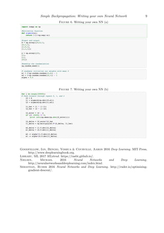
3. Writing your own NN
Sample python code to write your own NN is depicted in figure 6 and figure 7.
REFERENCES
Christopher, Bourez 2016 Neural Networks and Deep Learning.
http://christopher5106.github.io/deep/learning/2016/09/16/about-loss-functions-
multinomial-logistic-logarithm-cross-entropy-square-errors-euclidian-absolute-frobenius-
hinge.html.

9. Simple Backpropagation: Writing your own Neural Network 9
Figure 6. Writing your own NN (a)
Figure 7. Writing your own NN (b)
Goodfellow, Ian, Bengio, Yoshua & Courville, Aaron 2016 Deep Learning. MIT Press,
http://www.deeplearningbook.org.
Library, ML 2017 MLxtend. https://rasbt.github.io/.
Nielsen, Michael 2016 Neural Networks and Deep Learning.
http://neuralnetworksanddeeplearning.com/index.html.
Sebastian, Ruder 2016 Neural Networks and Deep Learning. http://ruder.io/optimizing-
gradient-descent/.