Download as PDF, PPTX
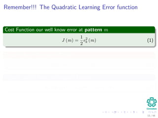


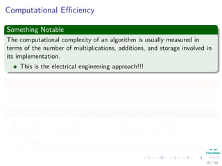
![Computational Efficiency
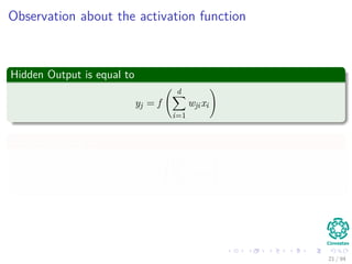
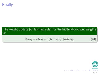
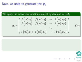
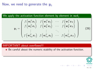
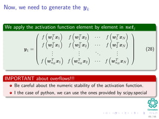
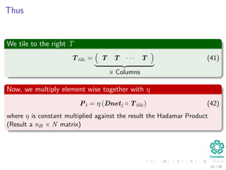
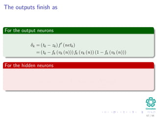
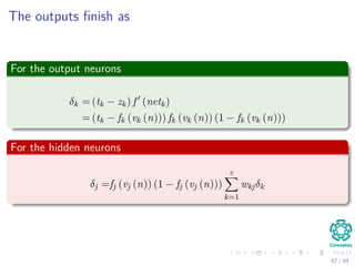
Now the Forward Pass
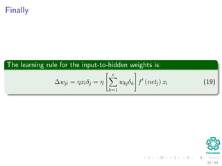
∆wji = ηxiδj = ηf (netj)
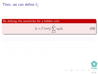
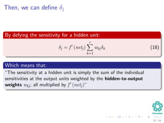
c
k=1
wkjδk xi
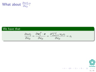
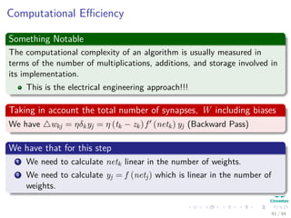
We have that for this step
[ c
k=1 wkjδk] takes, because of the previous calculations of δk’s, linear on
the number of weights
Clearly all this takes to have memory
In addition the calculation of the derivatives of the activation functions,
but assuming a constant time.
92 / 94](https://image.slidesharecdn.com/07-151212040333/85/15-Machine-Learning-Multilayer-Perceptron-207-320.jpg)
![Computational Efficiency
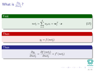
Now the Forward Pass
∆wji = ηxiδj = ηf (netj)
c
k=1
wkjδk xi
We have that for this step
[ c
k=1 wkjδk] takes, because of the previous calculations of δk’s, linear on
the number of weights
Clearly all this takes to have memory
In addition the calculation of the derivatives of the activation functions,
but assuming a constant time.
92 / 94](https://image.slidesharecdn.com/07-151212040333/85/15-Machine-Learning-Multilayer-Perceptron-208-320.jpg)
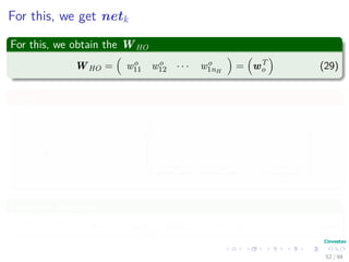
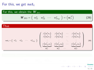
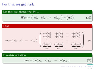
![Computational Efficiency
Now the Forward Pass
∆wji = ηxiδj = ηf (netj)
c
k=1
wkjδk xi
We have that for this step
[ c
k=1 wkjδk] takes, because of the previous calculations of δk’s, linear on
the number of weights
Clearly all this takes to have memory
In addition the calculation of the derivatives of the activation functions,
but assuming a constant time.
92 / 94](https://image.slidesharecdn.com/07-151212040333/85/15-Machine-Learning-Multilayer-Perceptron-209-320.jpg)
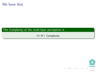

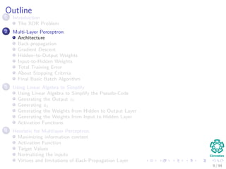
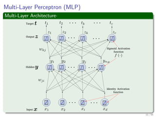
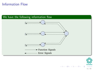
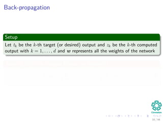
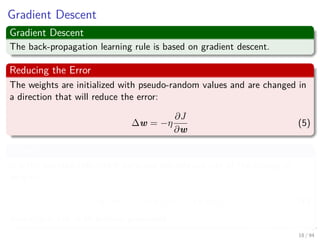
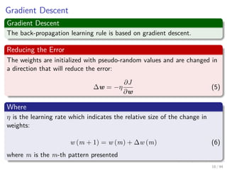
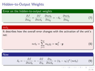
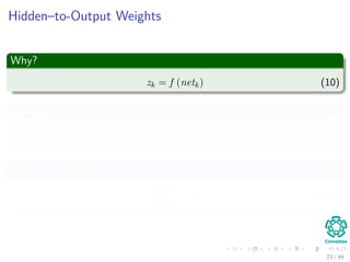
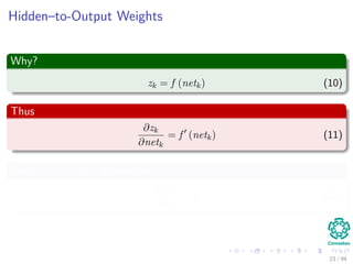
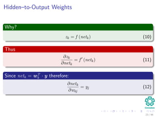
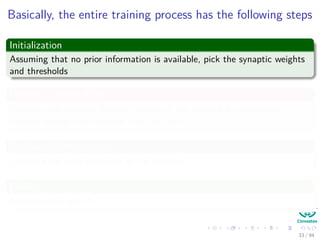
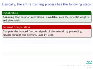
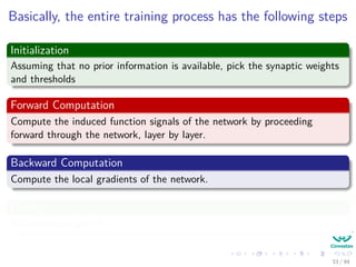
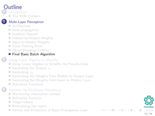
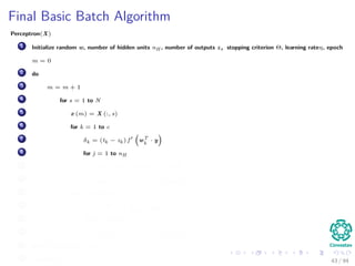
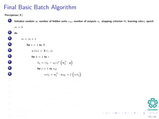
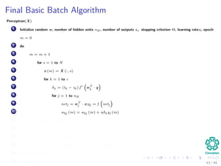
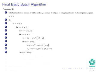
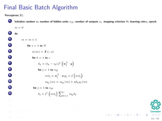
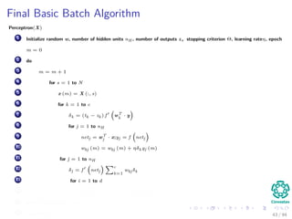
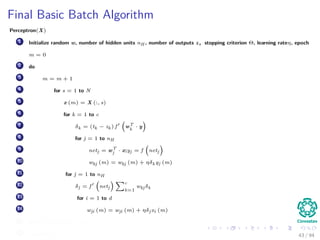
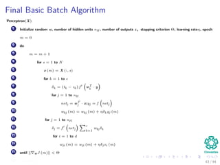
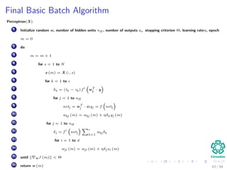
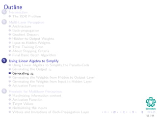
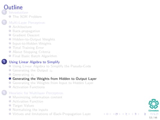
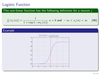
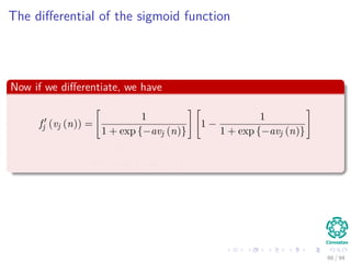
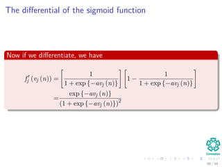
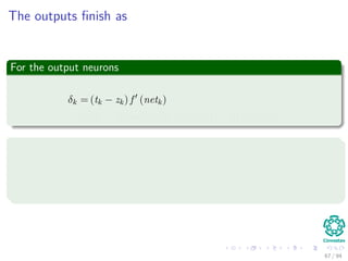
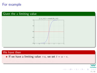
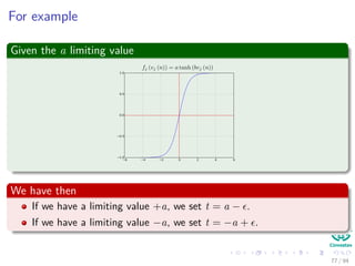
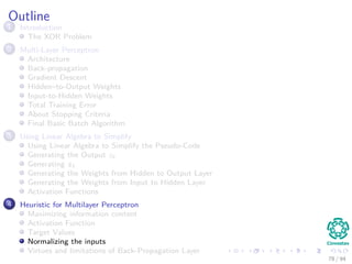
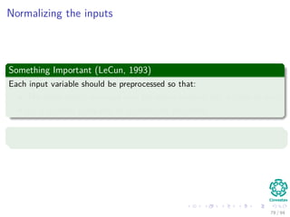
The document provides an overview of multi-layer perceptrons (MLPs) and details the back-propagation algorithm, highlighting its importance in training neural networks to solve complex problems like the XOR challenge. It discusses the architecture of MLPs, including weight initialization, activation functions, and the gradient descent method used for minimizing error during training. Additionally, the document touches on the historical context of back-propagation and its resurgence in recent years due to advancements in computational power.