This document summarizes a presentation on deep neural networks and computational graphs. It discusses how neural networks work using an example of a network with inputs, hidden layers, and an output. It also explains key concepts like activation functions, backpropagation for updating weights, and how the chain rule is applied in backpropagation. Computational graphs are introduced as a way to represent mathematical expressions and evaluate gradients to train neural networks.

1. Deep Neural Networks & Computational Graphs
By
P Revanth Kumar
Research Scholar,
IFHE Hyderabad.

2. Objective
• To improve the performance of a Deep Learning model. The goal is to the
reduce the optimization function which can be divided based on the
classification and the regression problems.

3. Agenda
• Deep Learning
• How Neural Network Work
• Activation function
• Neural Network with Back Propagation
• What is Chain rule
• Chain rule in back propagation
• Computation Graph

4. Deep Learning
• Deep learning is a technique which basically mimics the human brain.
• So, the Scientist and Researchers taught can we make machine learn in the
same way so, their is where deep learning concept came that lead to the
invention called neural network.
• The 1st simplest type of neural network is called perceptron.
• There was some problems in the perceptron because the perceptron not
able to learn properly because the concepts they applied.
• But later on in 1980’s Geoffrey Hinton he invented concept called
backpropagation. So, the ANN, CNN, RNN became efficient that many
companies are using it, developed lot of applications.

5. • 𝑓1, 𝑓2, 𝑓3 are my input features
• This resembles the ANN
• If it is a multi classification: more than one node can be specified
• If it is a binary classification: only one node need to be specified

6. How Neural Network Work
• Features 𝑥1, 𝑥2, 𝑥3 for my input layer. I want to determine binary
classification.
• Now, let us understand what kind of process does hidden layer do and
what is the importance of 𝑤1, 𝑤2, 𝑤3 (weights).

7. • As soon as the inputs are given they will get multiplied with respective
weights which are intern inputs for hidden layer
• The activation function will trigger.
• When 𝑤1, 𝑤2, 𝑤3 are assigned, the weights passes to the hidden neuron.
Then two types of operation usually happen.
• Step 1: The summation of weights and the inputs
i=1
n
WiXi
y= 𝑤1 𝑥1 + 𝑤2 𝑥2 + 𝑤3 𝑥3

8. • Step 2: Before activation function the bias will be added and summation
follows
y= 𝑤1 𝑥1 + 𝑤2 𝑥2 + 𝑤3 𝑥3+𝑏𝑖 (1)
z= Act (y) * Sigmoid function
z= z × 𝑤4
• If it is a classification problem then 0 or 1 will be obtained.
• This is an example of forward propagation.

9. Activation function
• The activation function is a mathematical “gate” in between the input
feeding the current neuron and its output going to the next layer. It can be
as simple as a step function that turns the neuron output on and off
depending on a rule or threshold.
• Sigmoid Function = σ 𝑋 =
1
1+𝑒−𝑦 ; y= 𝑖=1
𝑛
𝑊𝑖 𝑋𝑖+𝑏𝑖
• This will transform the value between 0 or 1. If it is < 0.5 considered as 0.
Here 0.5 is the threshold.

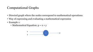
10. Neural Network with Back Propagation
• Let us consider a dataset
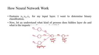
• Forward propagation: Let Inputs are 𝑥1, 𝑥2, 𝑥3. These inputs will pass to
neuron. Then 2 important operations will take place
y= [𝑤1 𝑥1 + 𝑤2 𝑥2 + 𝑤3 𝑥3]+𝑏𝑖
z= Act (y) * Sigmoid Activation function
𝒙 𝟏 𝒙 𝟐 𝒙 𝟑 O/P
Play Study Sleep y
2h 4h 8h 1
*Only one hidden neuron is considered for training example

11. • y is the predicted output; Suppose y is predicted as 0, but, we know that we
need to compare to check whether the y and y are almost same.
As current record y=1.
• The difference can be found by loss function
Loss = (𝑦 − 𝑦)2
= (1-0)2
= 1

12. • Here loss value is higher and completely predicted wrong.
• Now, the weights are to be adjusted in such a way that my predicted output
should be 1.
• This is basically done by using Optimizer. To reduce the loss value back
propagate need to be used.
Back Propagation: While doing back propagation these weights will get
w4new
= w4 𝑜𝑙𝑑
− α
𝜕L
𝜕w4

13. • Here learning rate α should be minimal value = 0.001.
• This small learning rate will help to reach global minima in the gradient
descent. Which is possible only with the optimizer.
• After updating 𝑤4, the other weights 𝑤1, 𝑤2, 𝑤3 need to be updated
respectively.
w3new
= w3 𝑜𝑙𝑑
− α
𝜕L
𝜕w3
• Once the values are updated, the forward propagation will start. It will
iterate to such a point the loss value will completely reduce to 𝑦 = 𝑦.
• Since there is a single record value defined with Loss function. If there are
multiple records the Cost function need to be defined.
i=1
n
(y − y)2

14. What is Chain Rule
• Chain Rule: Suppose u is a differentiable function of 𝑥1, 𝑥2, … 𝑥 𝑛 and each 𝑥𝑗 is a
differentiable function of 𝑡1 , 𝑡2, … 𝑡 𝑛. Then u is a function of 𝑡1 , 𝑡2, … 𝑡 𝑛 and the
the partial derivative u with respect to t is
𝜕𝑢
𝜕𝑡1
=
𝜕𝑢
𝜕𝑥1
𝜕𝑥1
𝜕𝑡1
+
𝜕𝑢
𝜕𝑥2
𝜕𝑥2
𝜕𝑡1
+ … +
𝜕𝑢
𝜕𝑥 𝑛
𝜕𝑥 𝑛
𝜕𝑡 𝑛

15. Chain Rule in Back Propagation
• Suppose the inputs are 𝑥1, 𝑥2, 𝑥3, 𝑥4 which are getting connected with two
hidden layers. In hidden layer one there are 3 neurons and in the hidden
layer two there 2 neurons.
• The best way to define the hidden layer is 𝑤11
1
for 1st hidden layer and 𝑤11
2
for the 2nd hidden layer.

16. • Let us update the weights; 𝑤11 𝑛𝑒𝑤
3
= 𝑤11 𝑜𝑙𝑑
3
− α
𝜕L
𝜕𝑤11
3
𝑤11
3
need to be updated in the back propagation, what we do is that we get a
𝑦 we get a loss value now, when we back propagate we update the weights.
• Now, we see how to find derivative 𝜕L
𝜕𝑤11
3 .This basically indicates the slope
and how it is related to chain rule.
•
𝜕L
𝜕𝑤11
3 can be written as
• The weight w11
3
will impact the output O31. Since it impact output 𝑂31 this
can be write as
𝜕L
𝜕𝑤11
3 =
𝜕𝐿
𝜕𝑂31
×
𝜕𝑂31
𝜕𝑤11
3 this is basically a chain rule

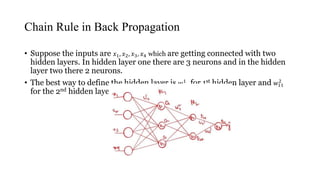
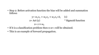
17. • Suppose, to find the derivative of w21
3
𝜕L
𝜕𝑤21
3 =
𝜕𝐿
𝜕𝑂31
×
𝜕𝑂31
𝜕𝑤21
3
• To find the derivative of w11
2
•
𝜕L
𝜕𝑤11
2 =
𝜕𝐿
𝜕𝑂31
×
𝜕𝑂31
𝜕𝑂21
×
𝜕𝑂21
𝜕𝑤11
2
• To find 𝑤12
2
because there are 2 output layers are impacting 𝑓21, 𝑓22.
• After finding the derivative adding one more derivative [
𝜕𝐿
𝜕𝑂31
×
𝜕𝑂31
𝜕𝑂21
×
𝜕𝑂21
𝜕𝑤11
2 ] +
[
𝜕𝐿
𝜕𝑂31
×
𝜕𝑂31
𝜕𝑂22
×
𝜕𝑂22
𝜕𝑤12
2 ]
• When this derivative is updated basically weights are getting updated then
𝑦 going to change until we reach global minima.

18. Computational Graphs
• Directed graph where the nodes correspond to mathematical operations.
• Way of expressing and evaluating a mathematical expression
• Example 1:
• Mathematical Equation: p = x + y
+
x
y
p

19. Back Propagation Algorithm
• Objective : Compute the gradients for each input with respect to the final
output.
• These gradients are essential for training the neural network using
gradient descent.
Desired Gradients:
𝜕𝑥
𝜕𝑓
,
𝜕𝑦
𝜕𝑓
,
𝜕𝑧
𝜕𝑓
x, y, z are the inputs.
G is the output.

20. • Step 1:
- Finding the derivative of output with respect to output itself
- This will result to the identity derivation and value is equal to one
𝜕𝑔
𝜕𝑔
= 1
• Computational graph

21. • Step 2
- Backward pass through the “*” operation.
- Calculation of gradients at nodes p and z. Since g=p*z
We know that
𝜕𝑔
𝜕𝑧
= 𝑝;
𝜕𝑔
𝜕𝑝
= 𝑧
From forward pass we get p and z as 4 and -3.
Hence, 𝜕𝑔
𝜕𝑧
= 𝑝 = 4 (1)
𝜕𝑔
𝜕𝑝
= 𝑧 = -3 (2)
• Step 3
Calculation of gradients at x and y.
𝜕𝑔
𝜕𝑥
,
𝜕𝑔
𝜕𝑦

22. • From chain rule:
𝜕𝑔
𝜕𝑥
=
𝜕𝑔
𝜕𝑝
∗
𝜕𝑝
𝜕𝑥
𝜕𝑔
𝜕𝑦
=
𝜕𝑔
𝜕𝑝
∗
𝜕𝑝
𝜕𝑦
dg/dp = -3 from (2)
Hence p = x + y = 𝜕𝑝
𝜕𝑥
= 1;
𝜕𝑝
𝜕𝑦
= 3
For input x
𝜕𝑔
𝜕𝑥
=
𝜕𝑔
𝜕𝑝
∗
𝜕𝑝
𝜕𝑥
= -3*1 = -3
For input y
𝜕𝑔
𝜕𝑦
=
𝜕𝑔
𝜕𝑝
∗
𝜕𝑝
𝜕𝑦
= -3*-3 = 9