Downloaded 1,854 times
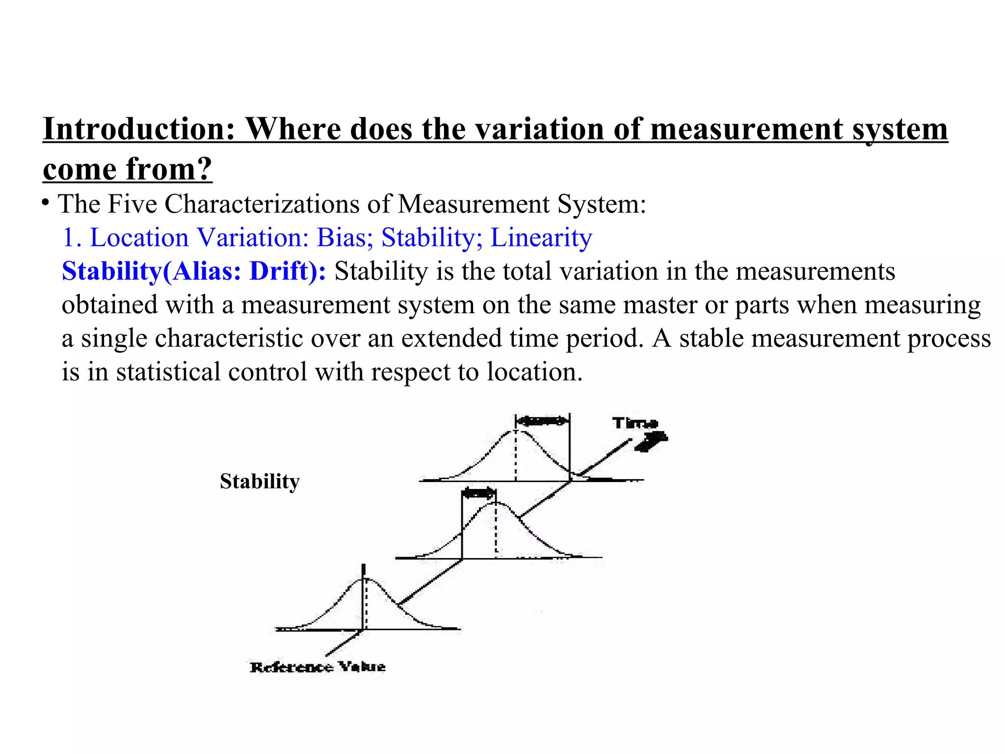
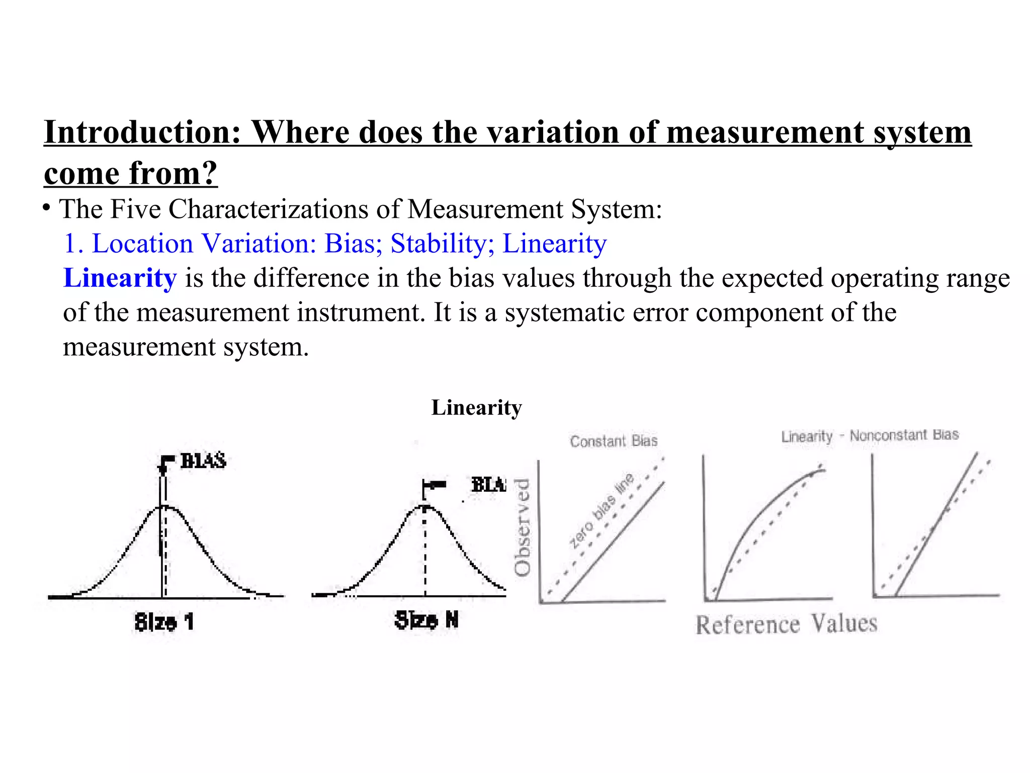
![Analysis Techniques: Variable Gage Analysis 8) Determine linearity and percent linearity: Linearity = Slope x Process variation( m ) %Linearity = 100[linearity/Process Variation] The acceptability criteria of Bias, Linearity depend on Quality Control Plan, characteristic being measured and gage speciality, suggested criteria of ESG is as following: Under 5% - acceptable 5% to 15% - may be acceptable based upon importance of application, cost of measurement device, cost of repairs, etc., Over 15% - Considered not acceptable - every effort should be made to improve the system The stability is determined through the use of a control chart. It is important to note that, when using control charts, one must not only watch for points that fall outside of the control limits, but also care other special cause signals such as trends and centerline hugging.Guideline for the detection of such signals can be found in many publications on SPC.](https://image.slidesharecdn.com/02trainingmaterialformsa-111030062223-phpapp02/75/02training-material-for-msa-33-2048.jpg)
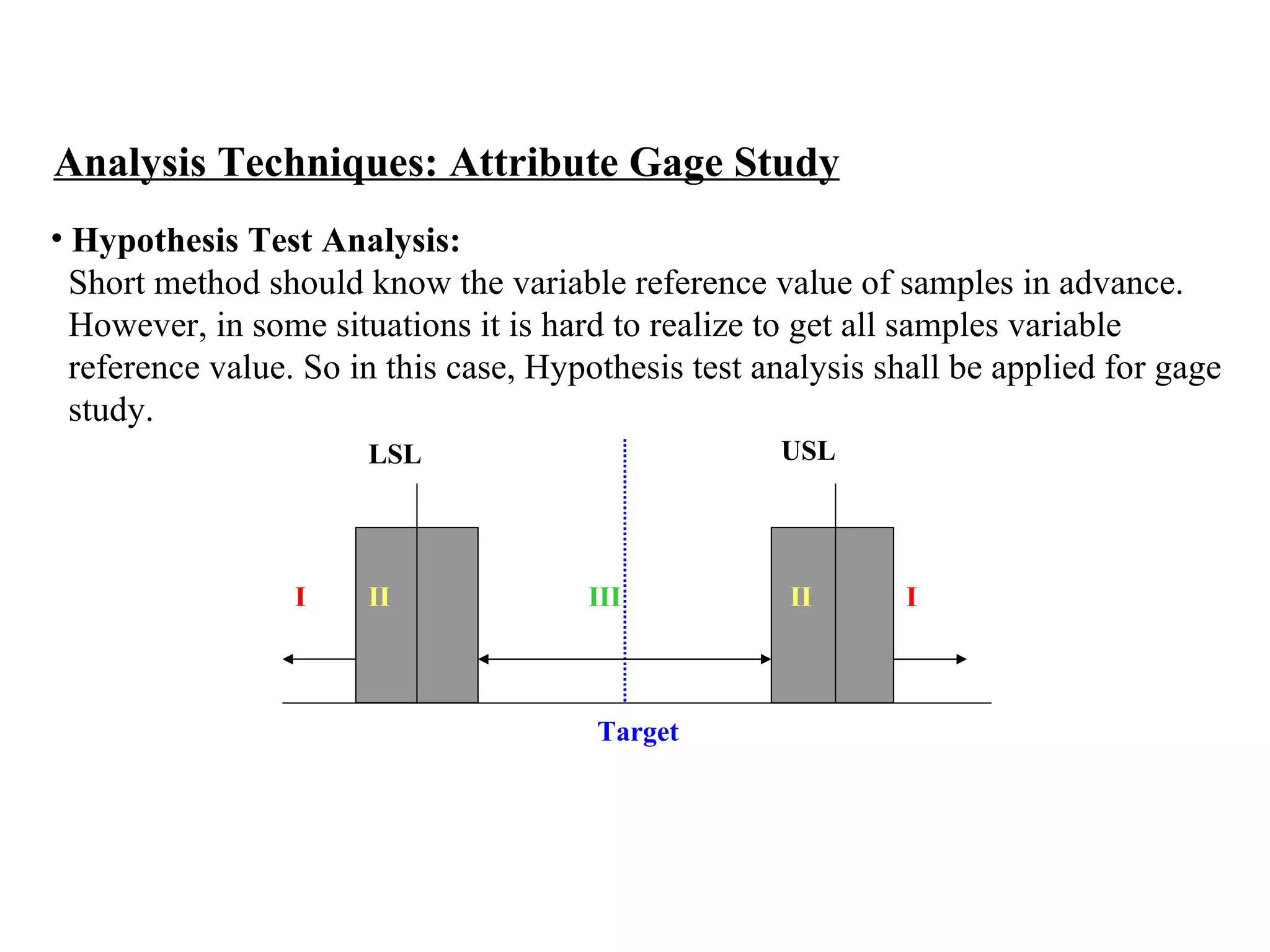
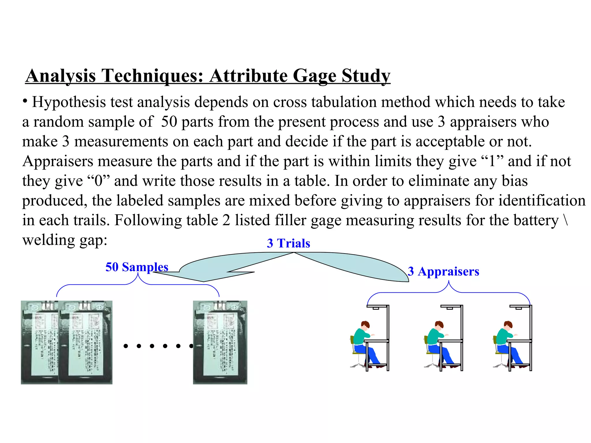
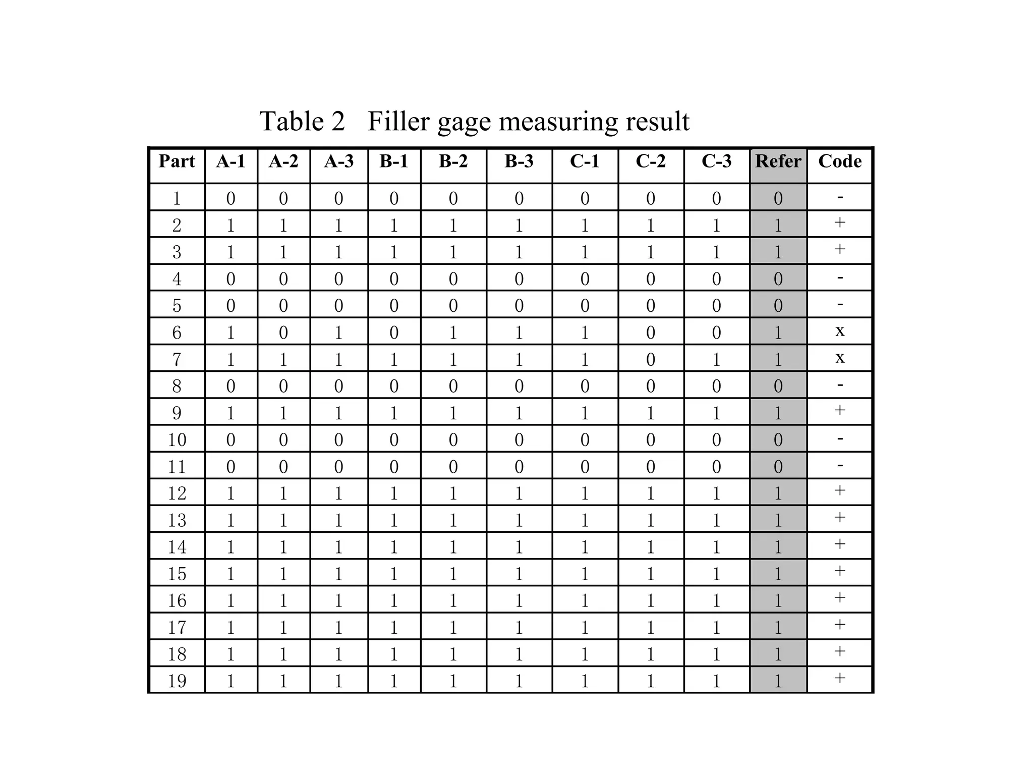
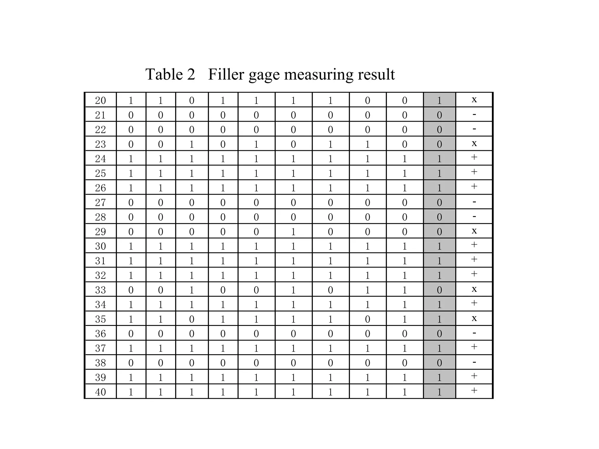
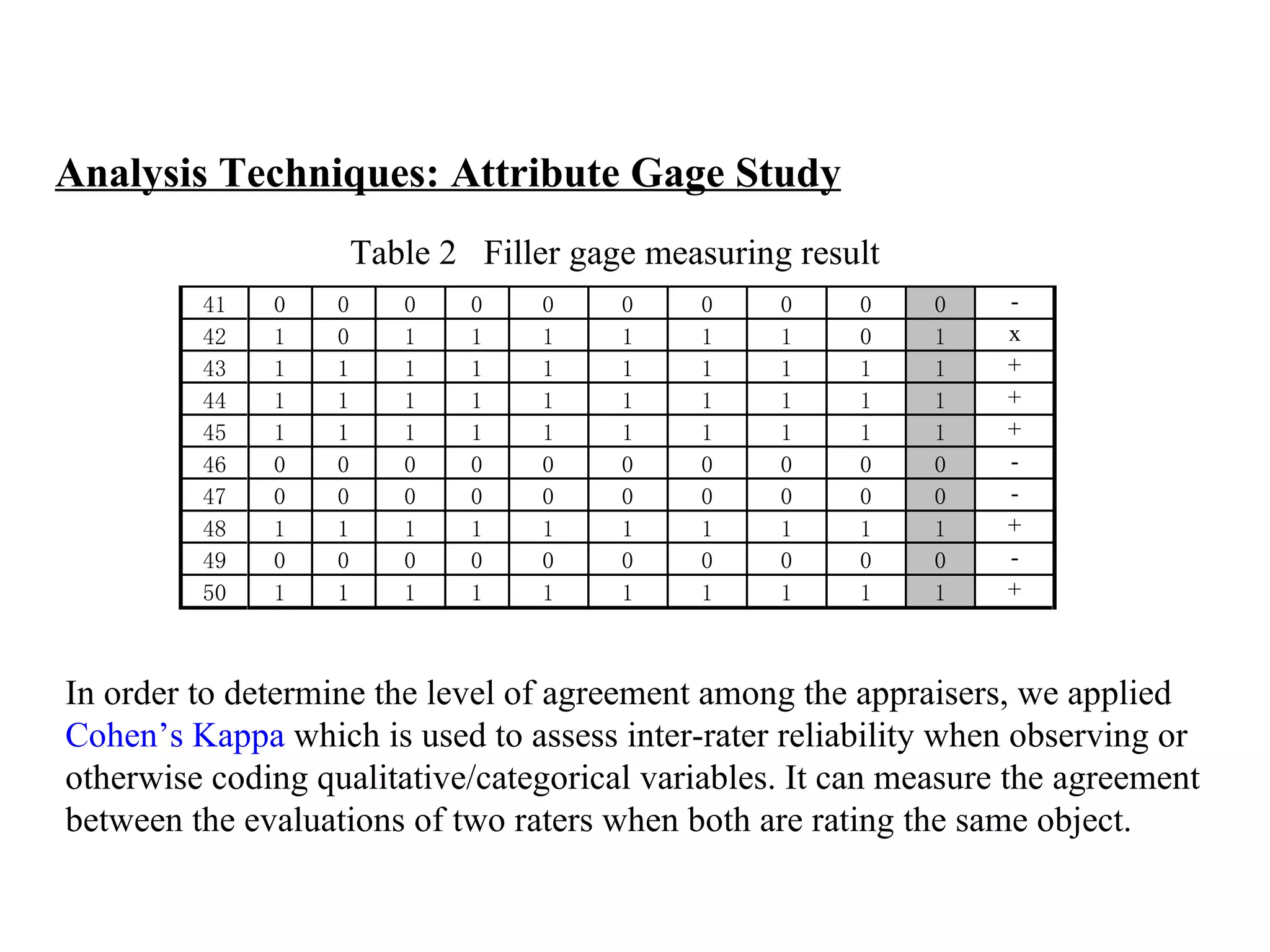
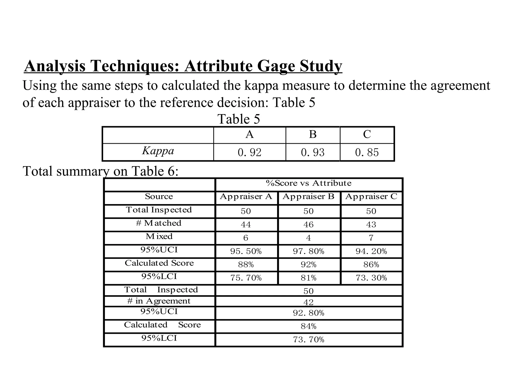
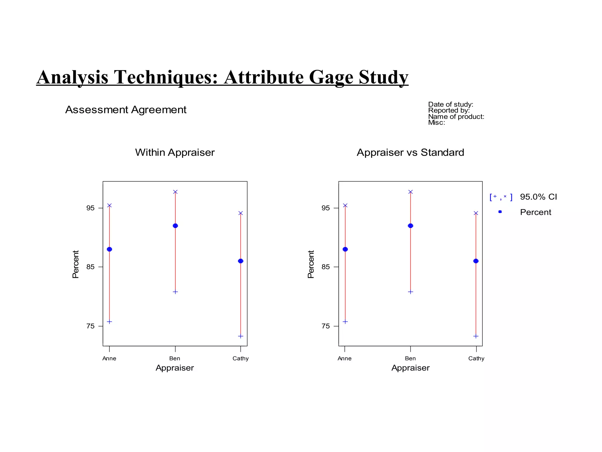
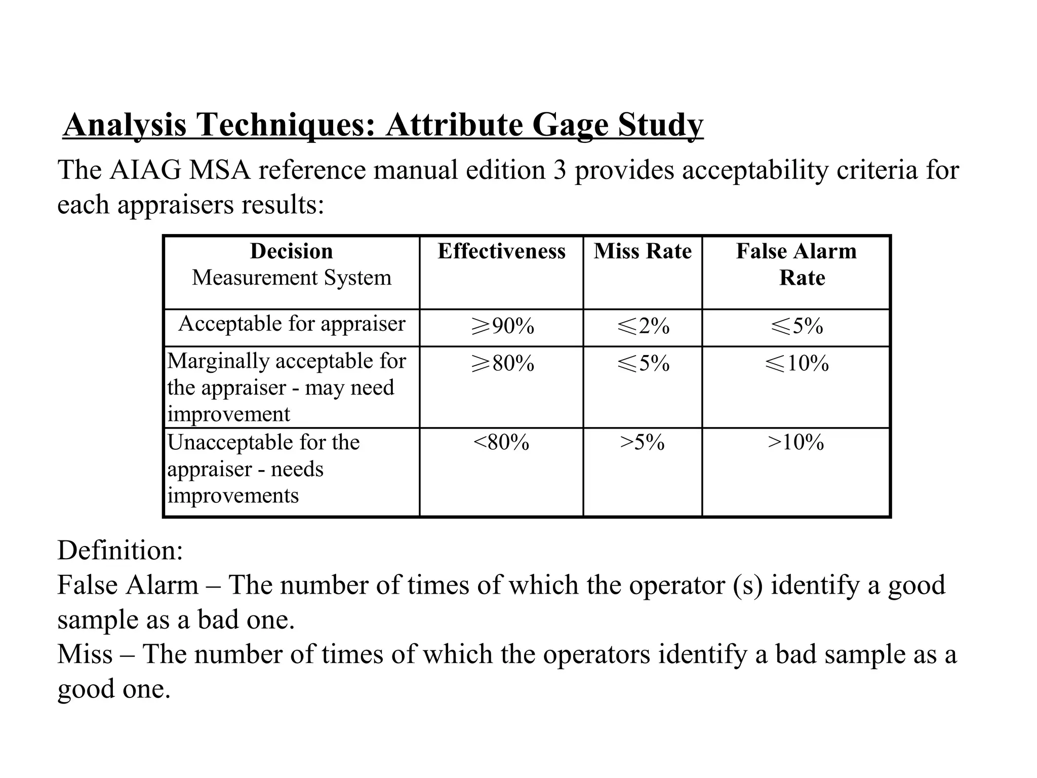
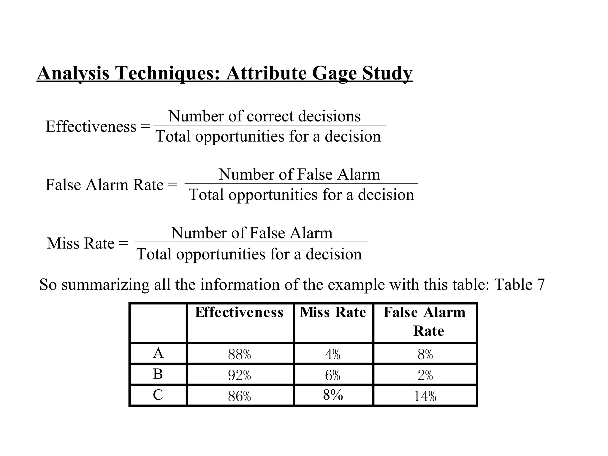
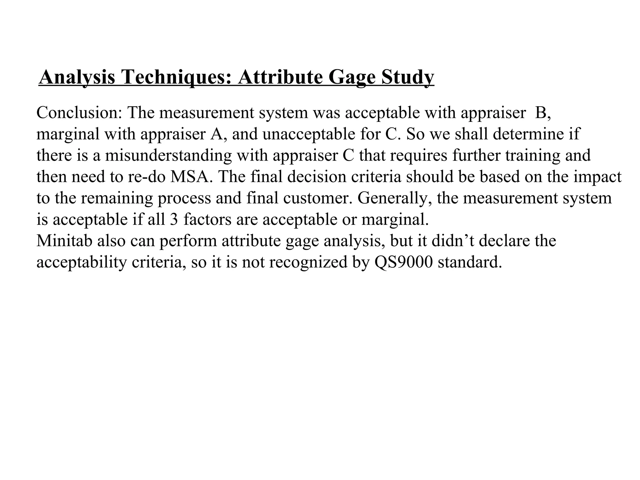
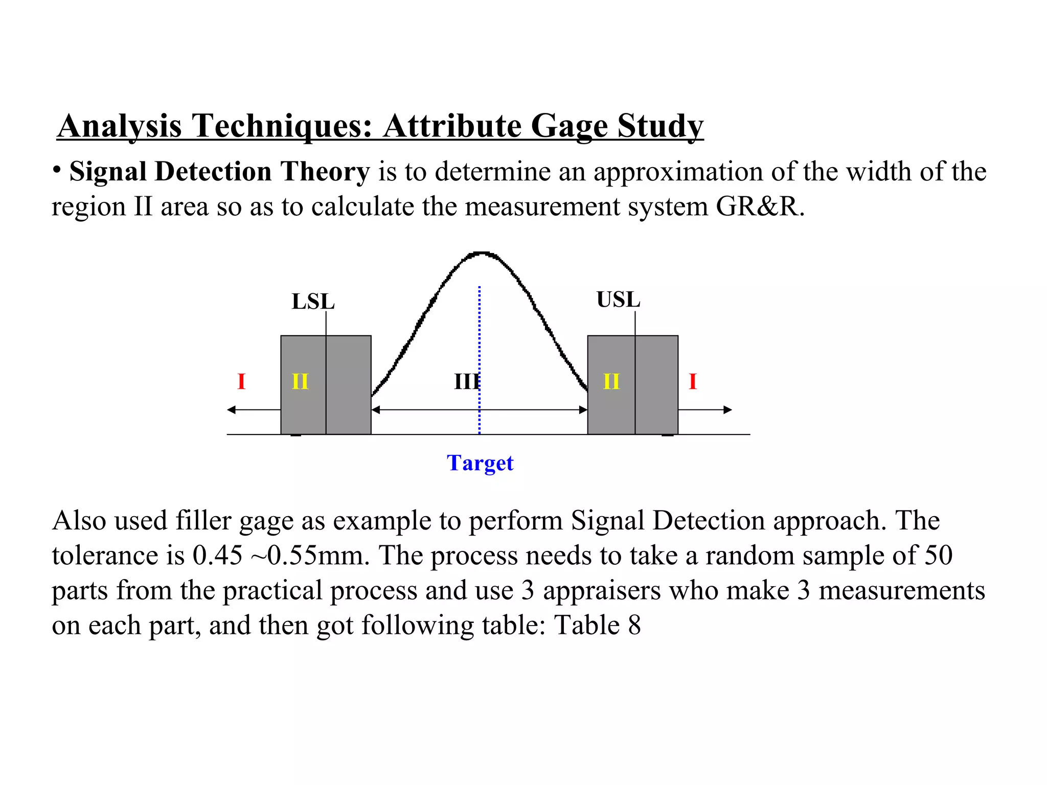
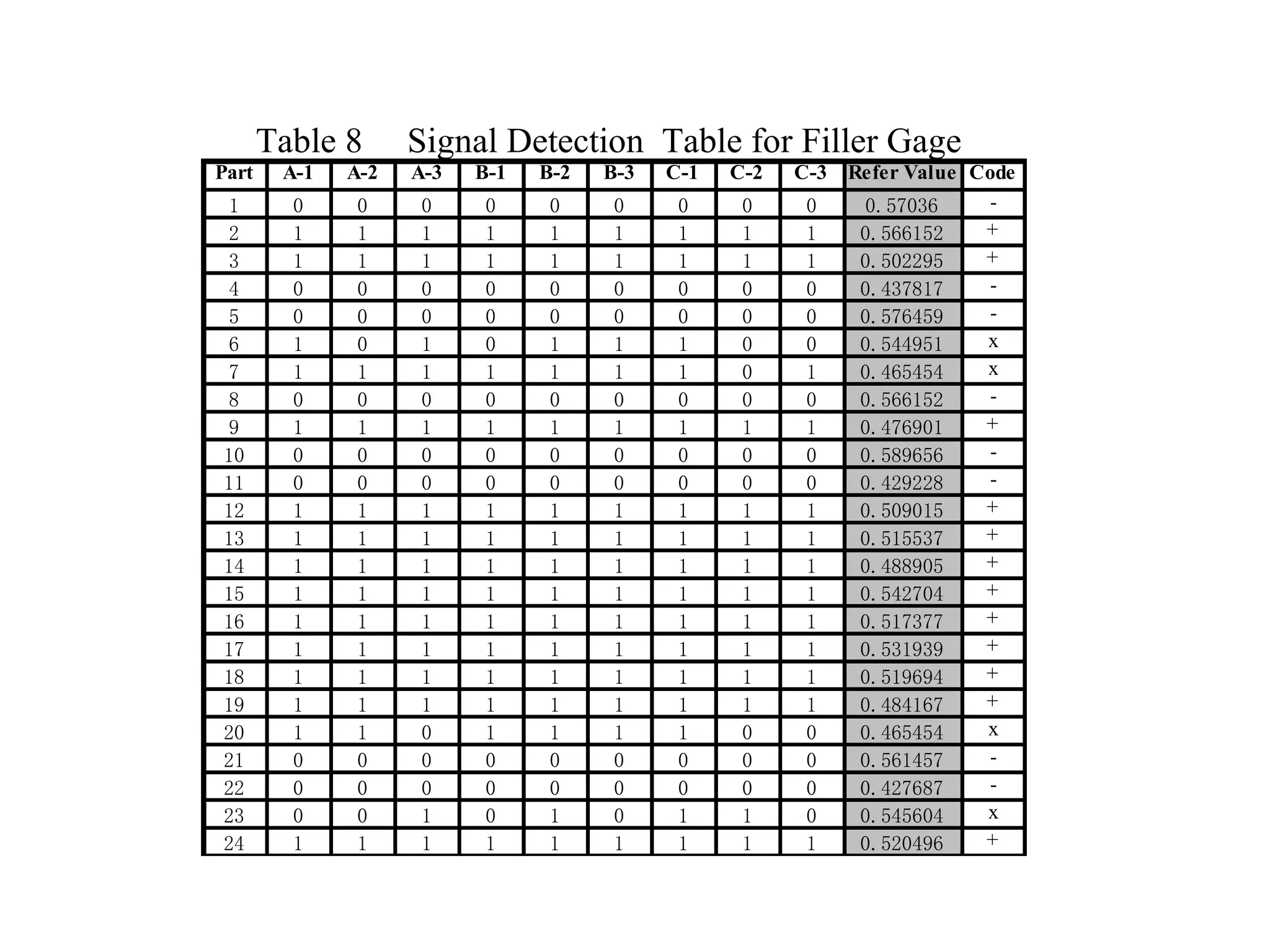
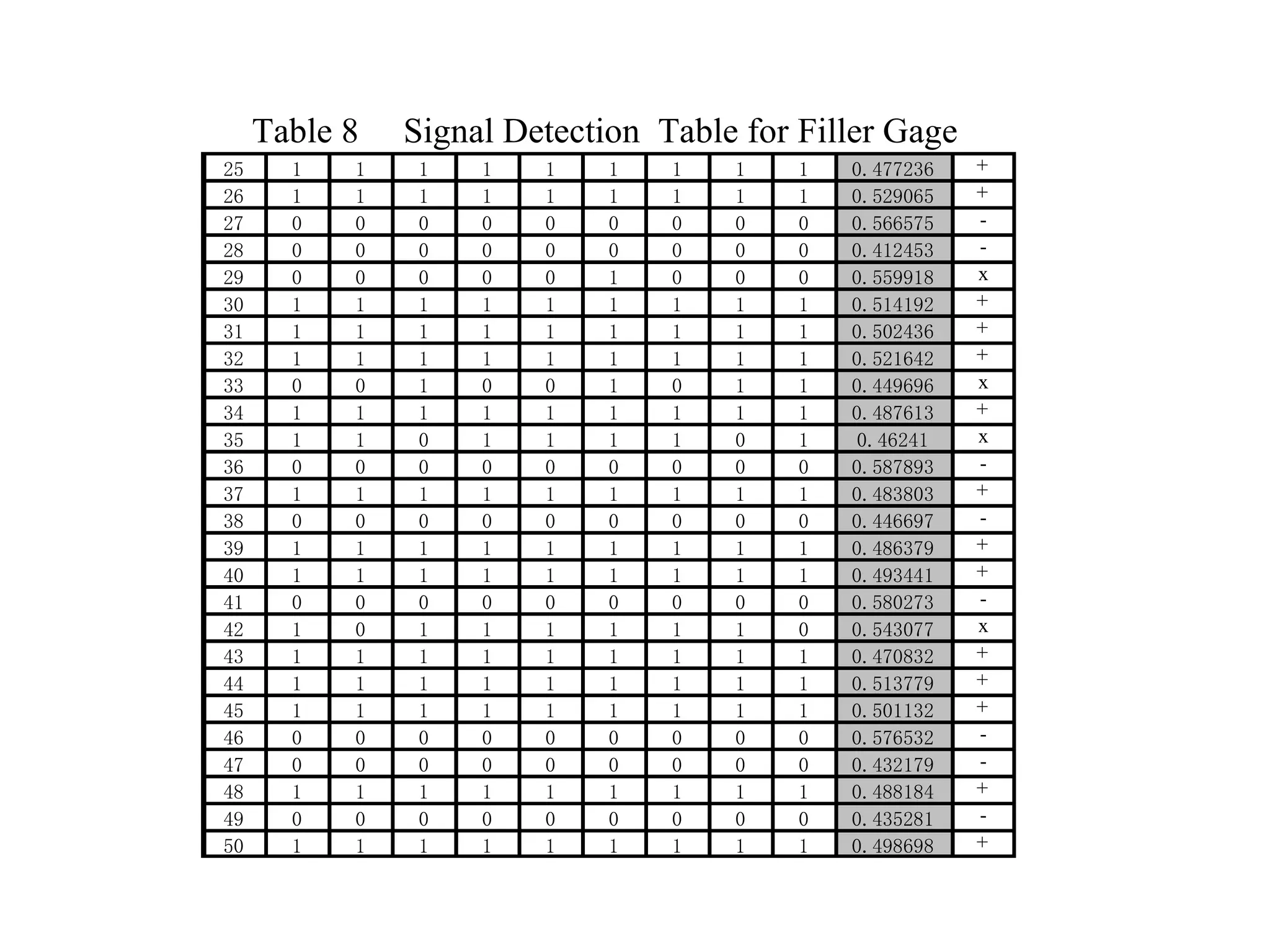
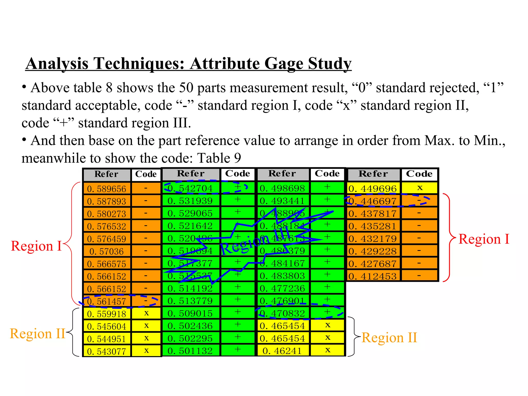
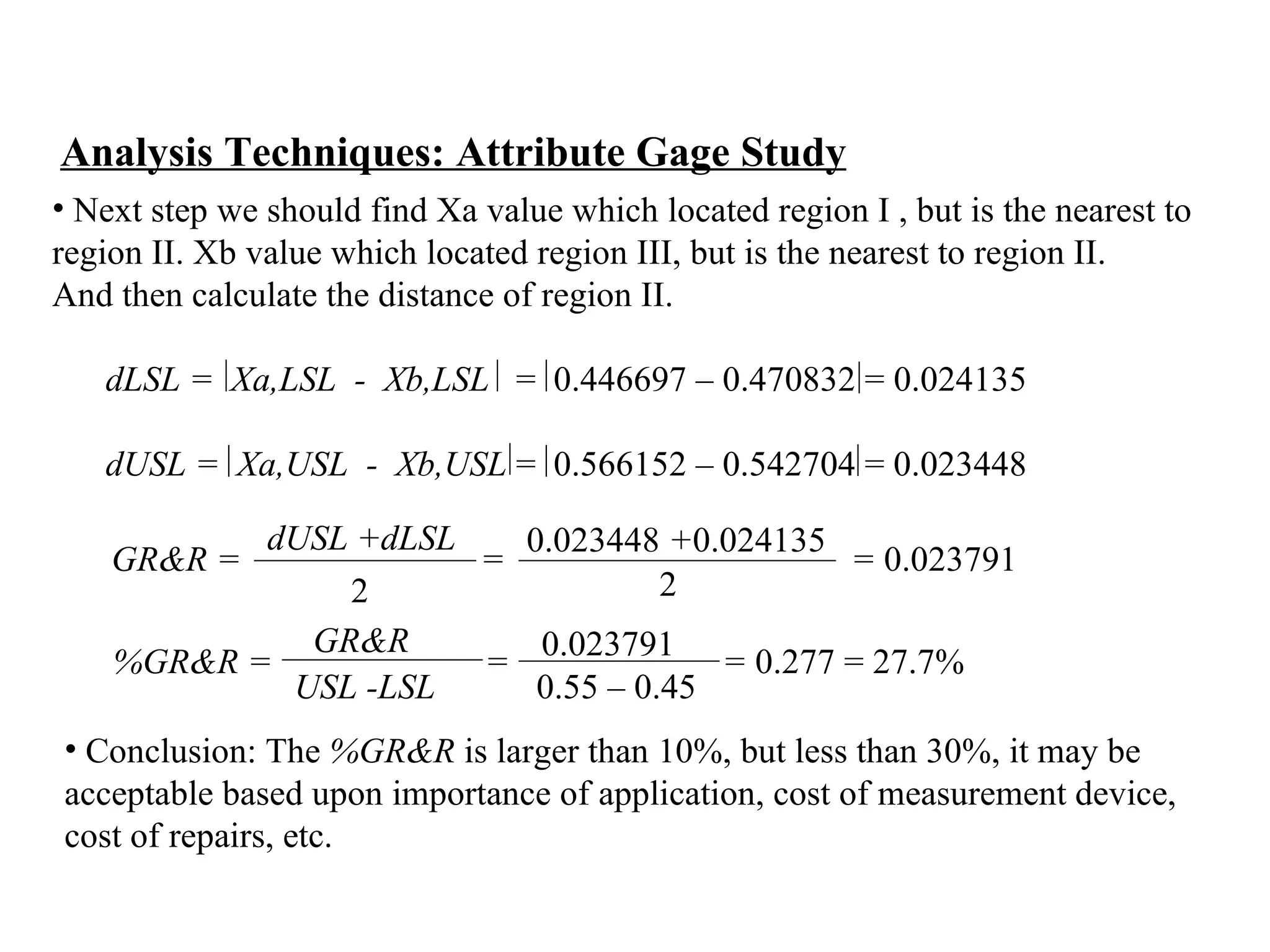
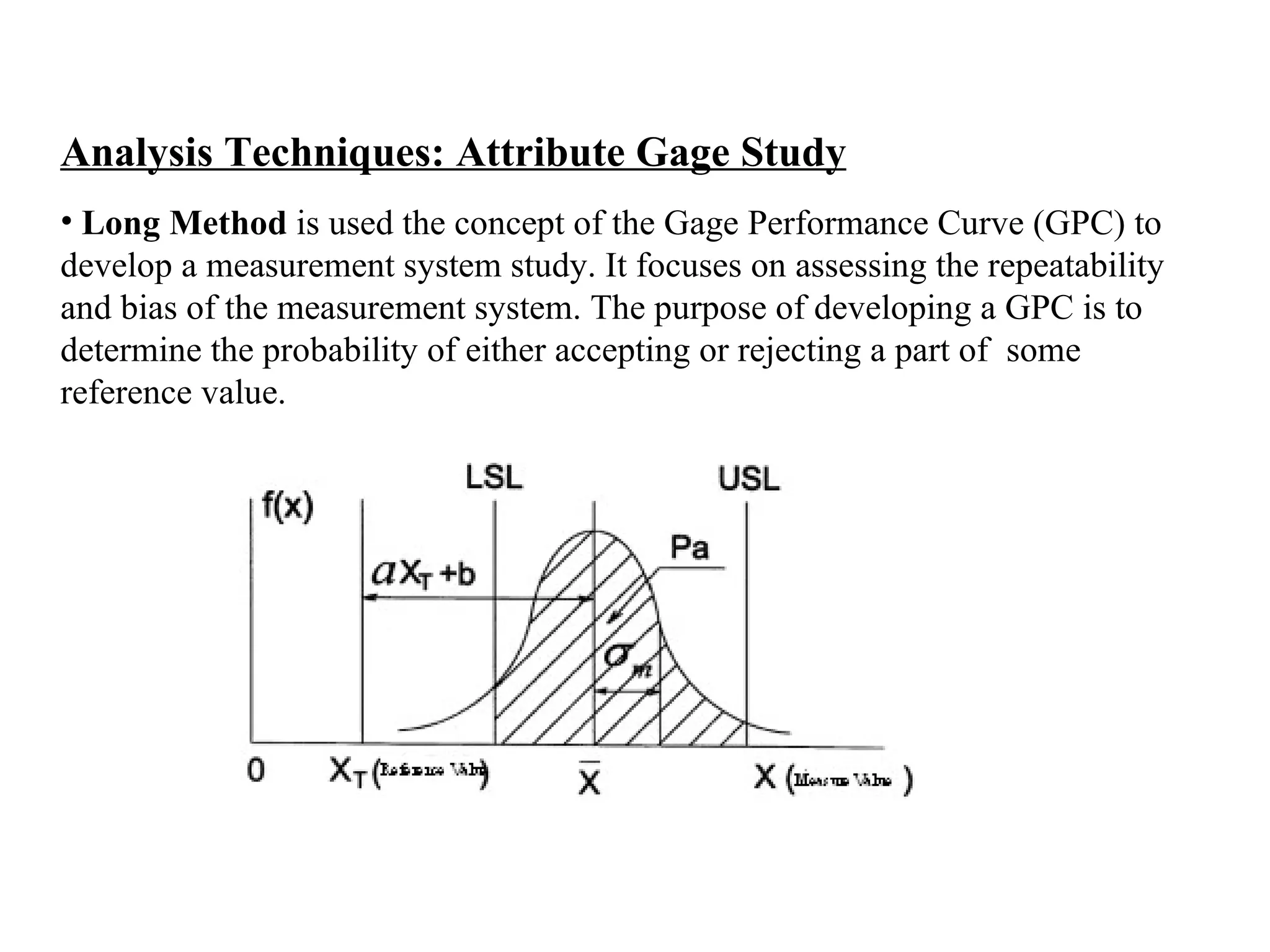
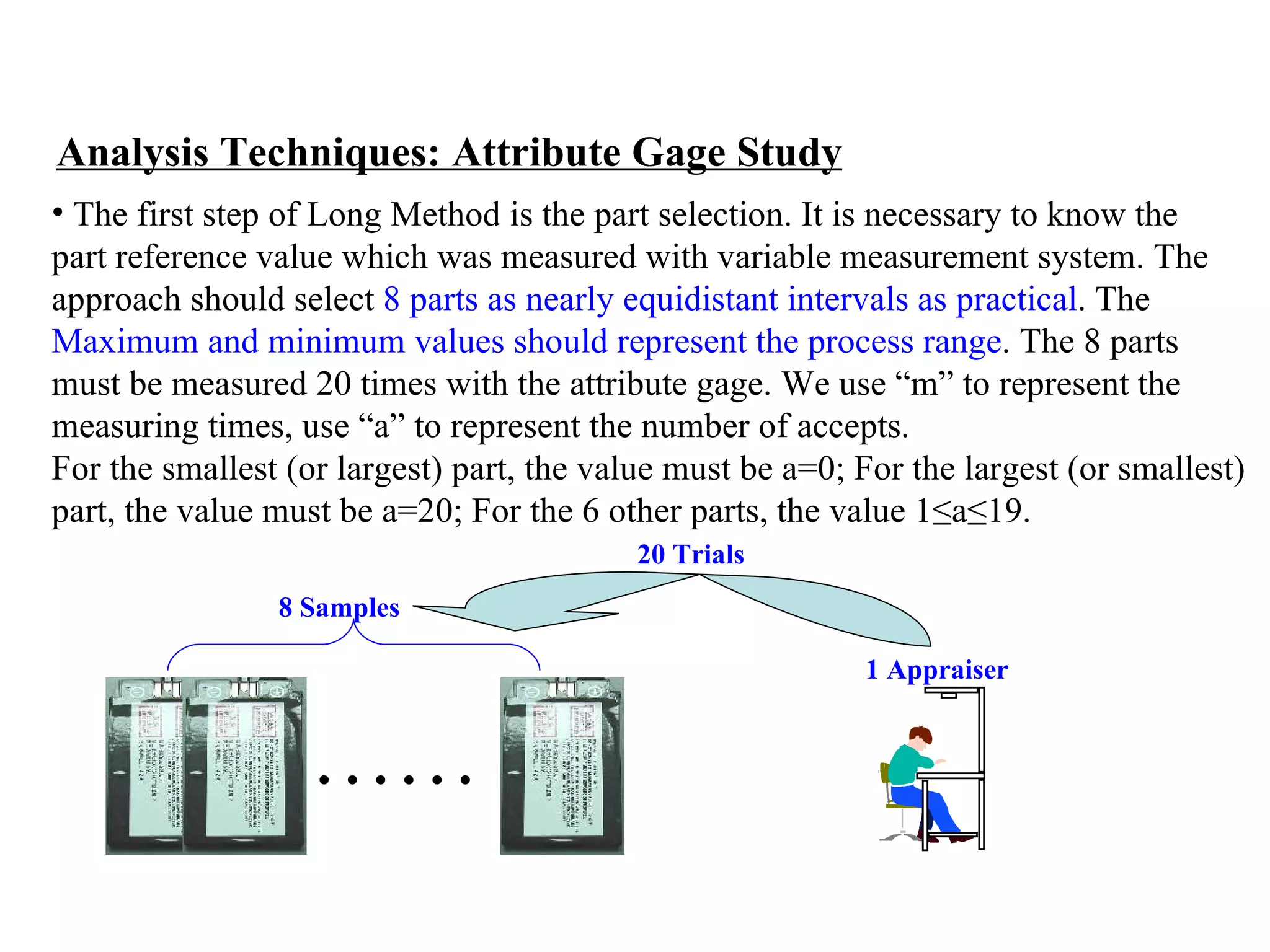
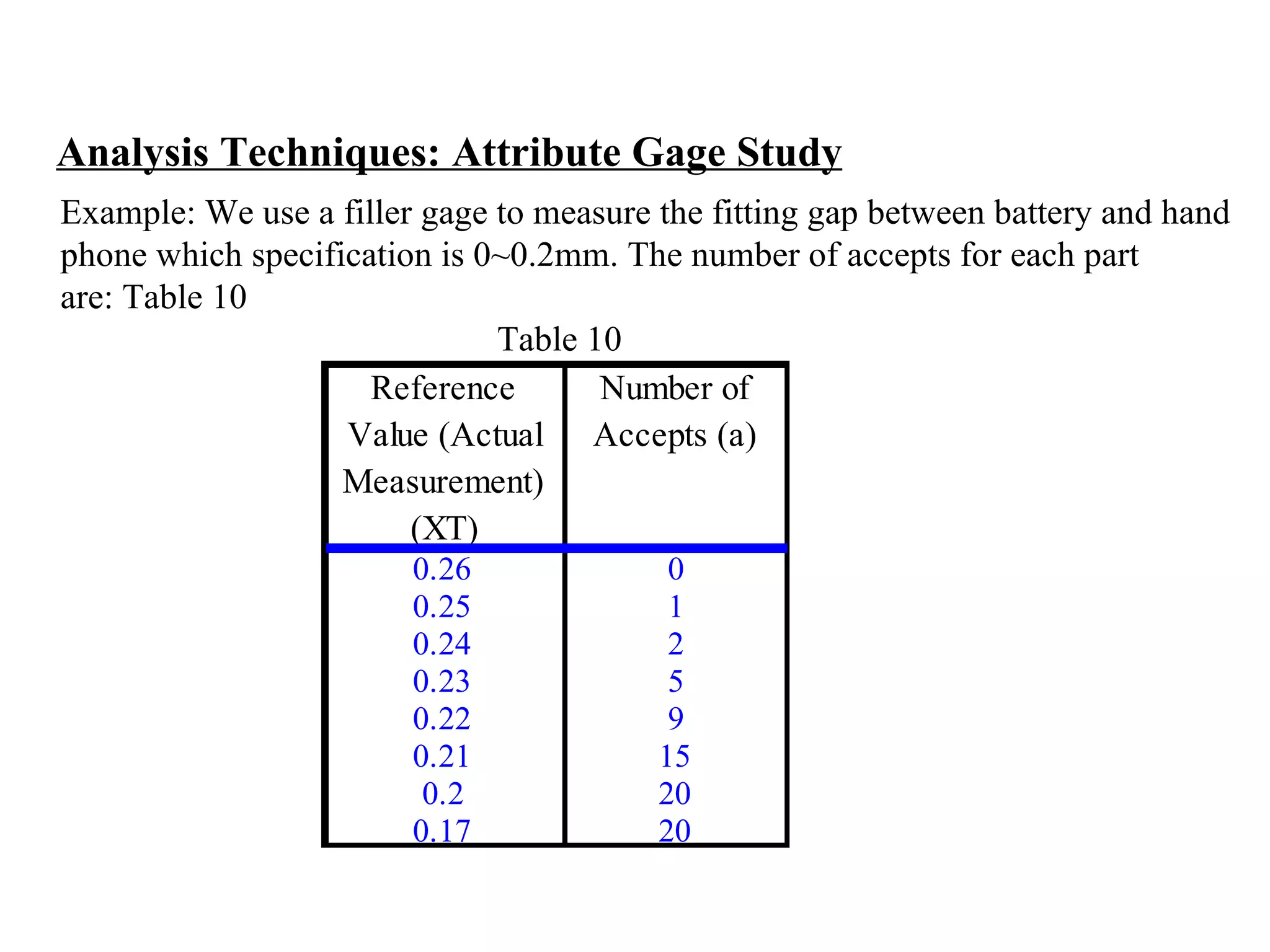
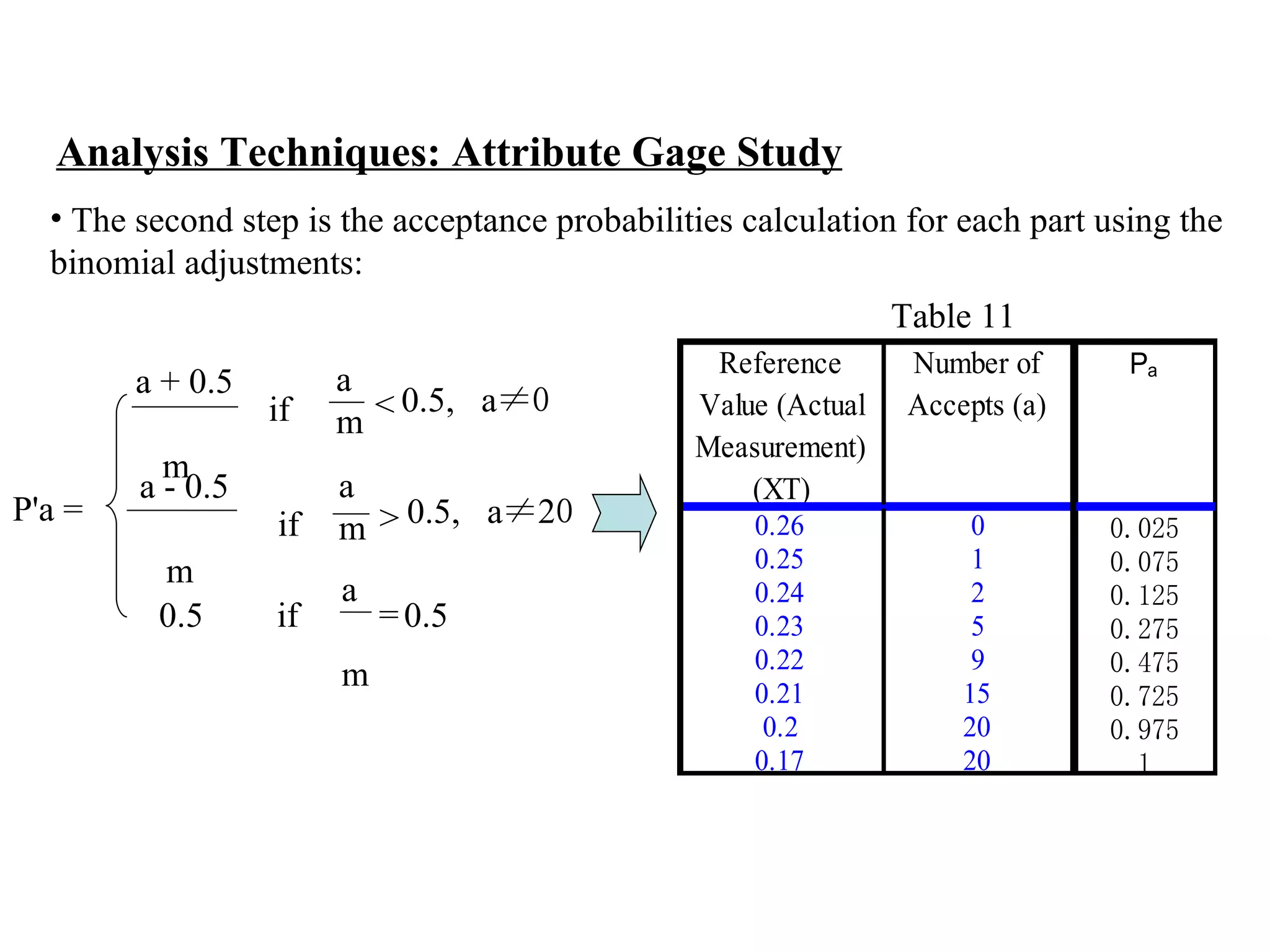
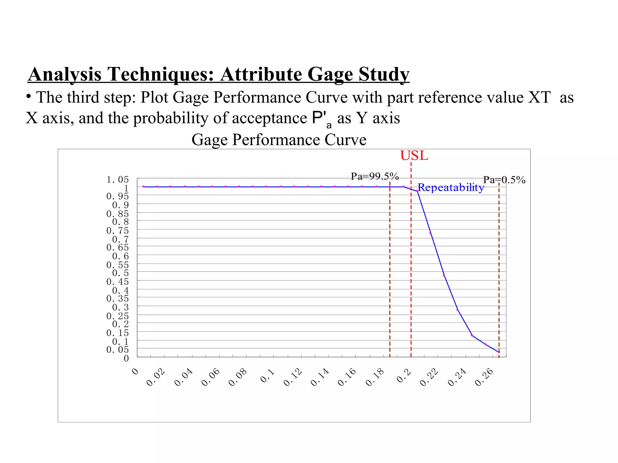
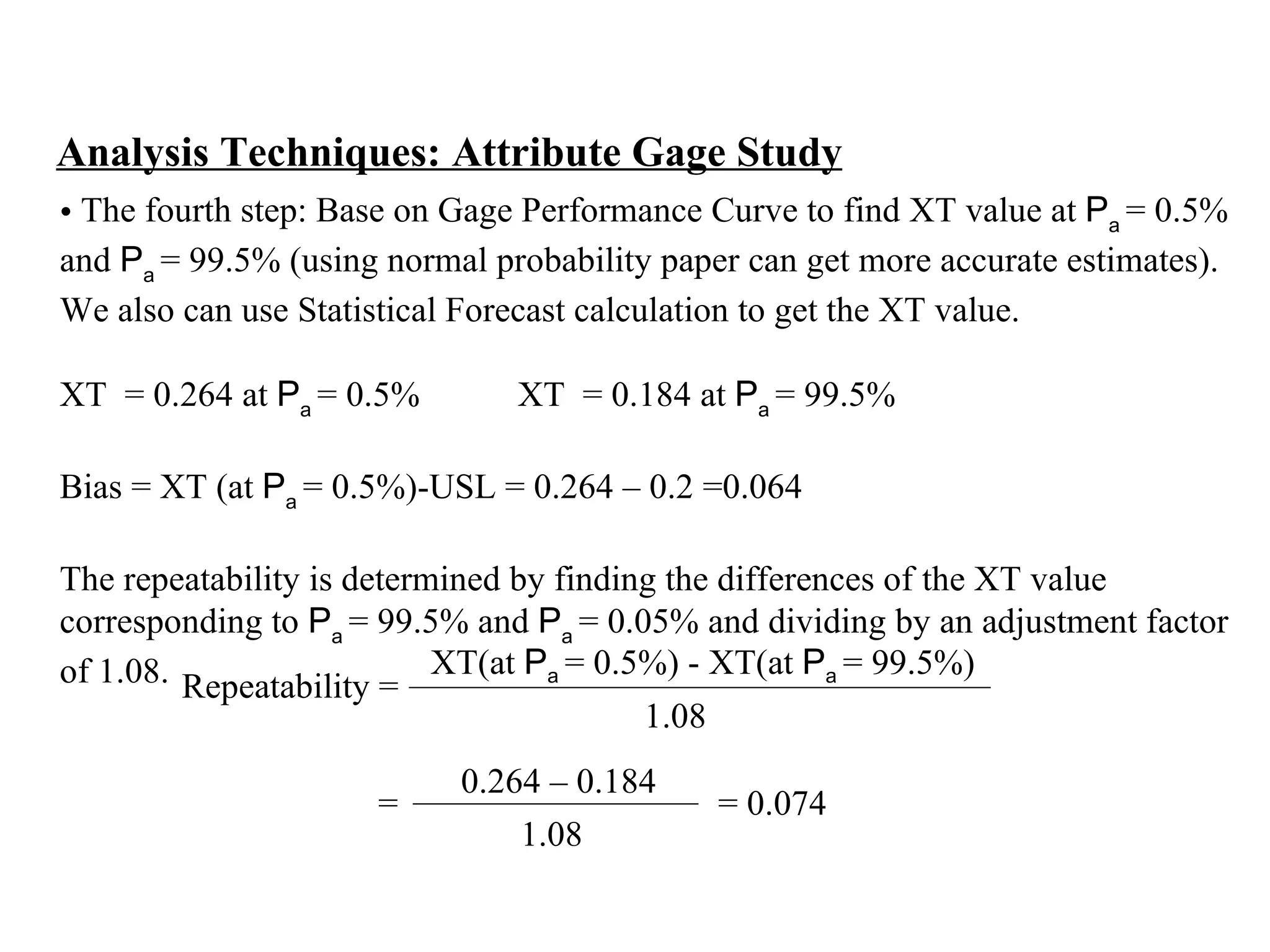

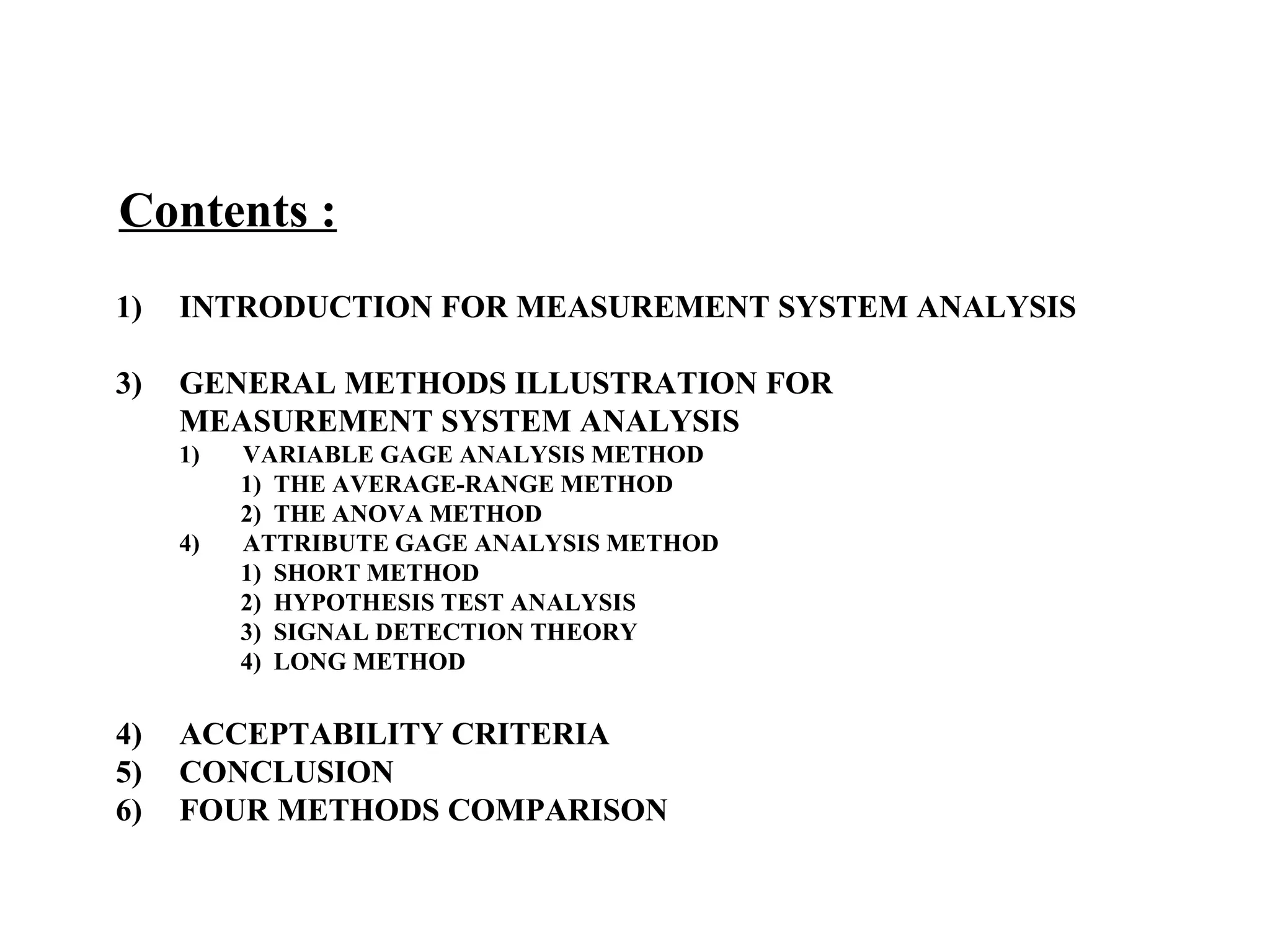
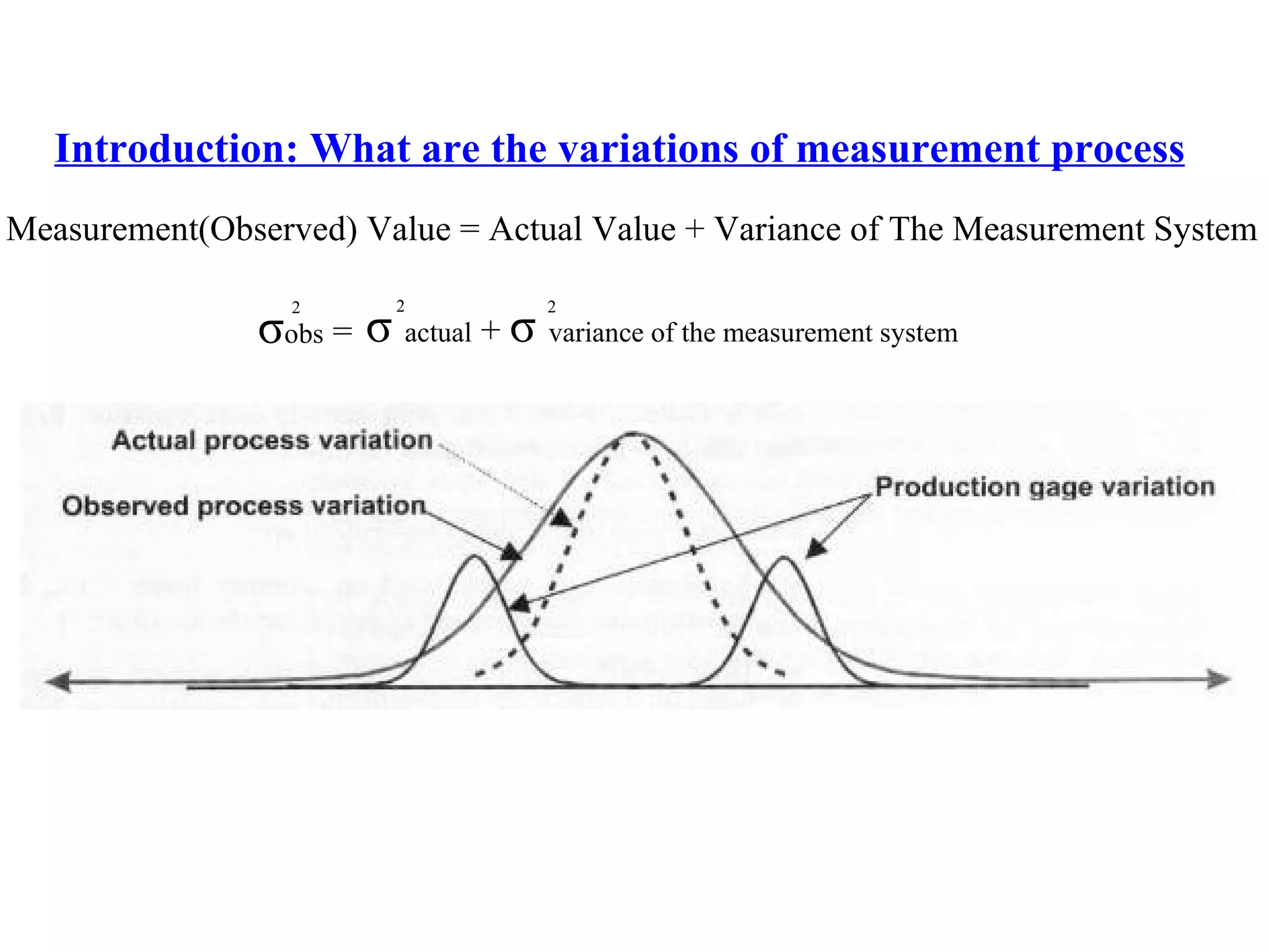
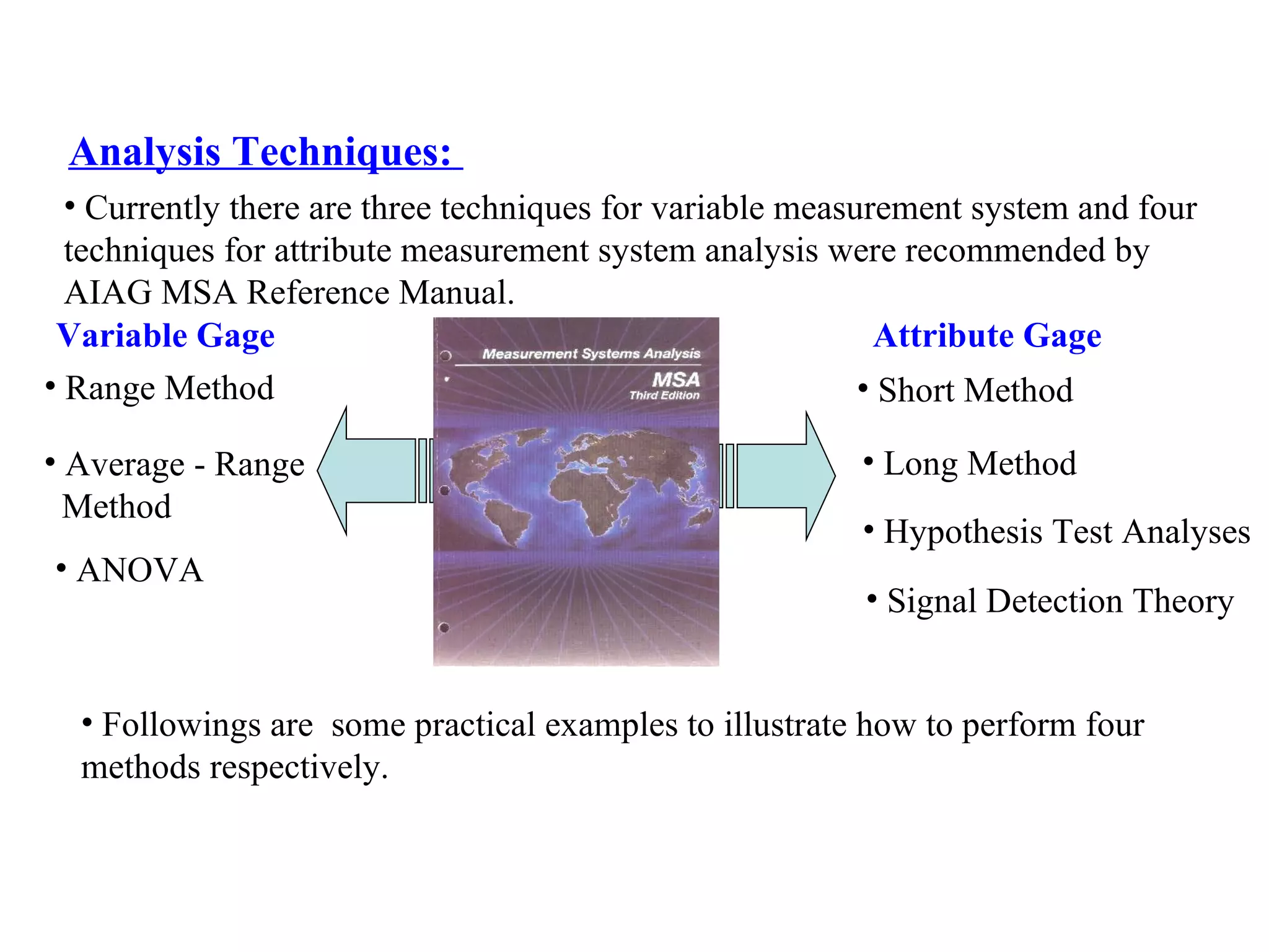
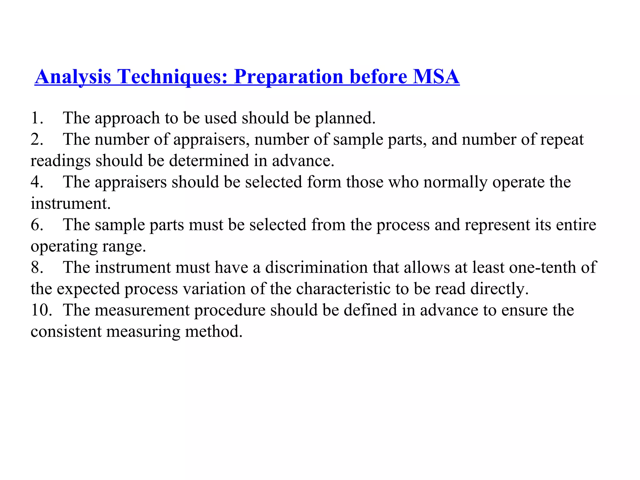
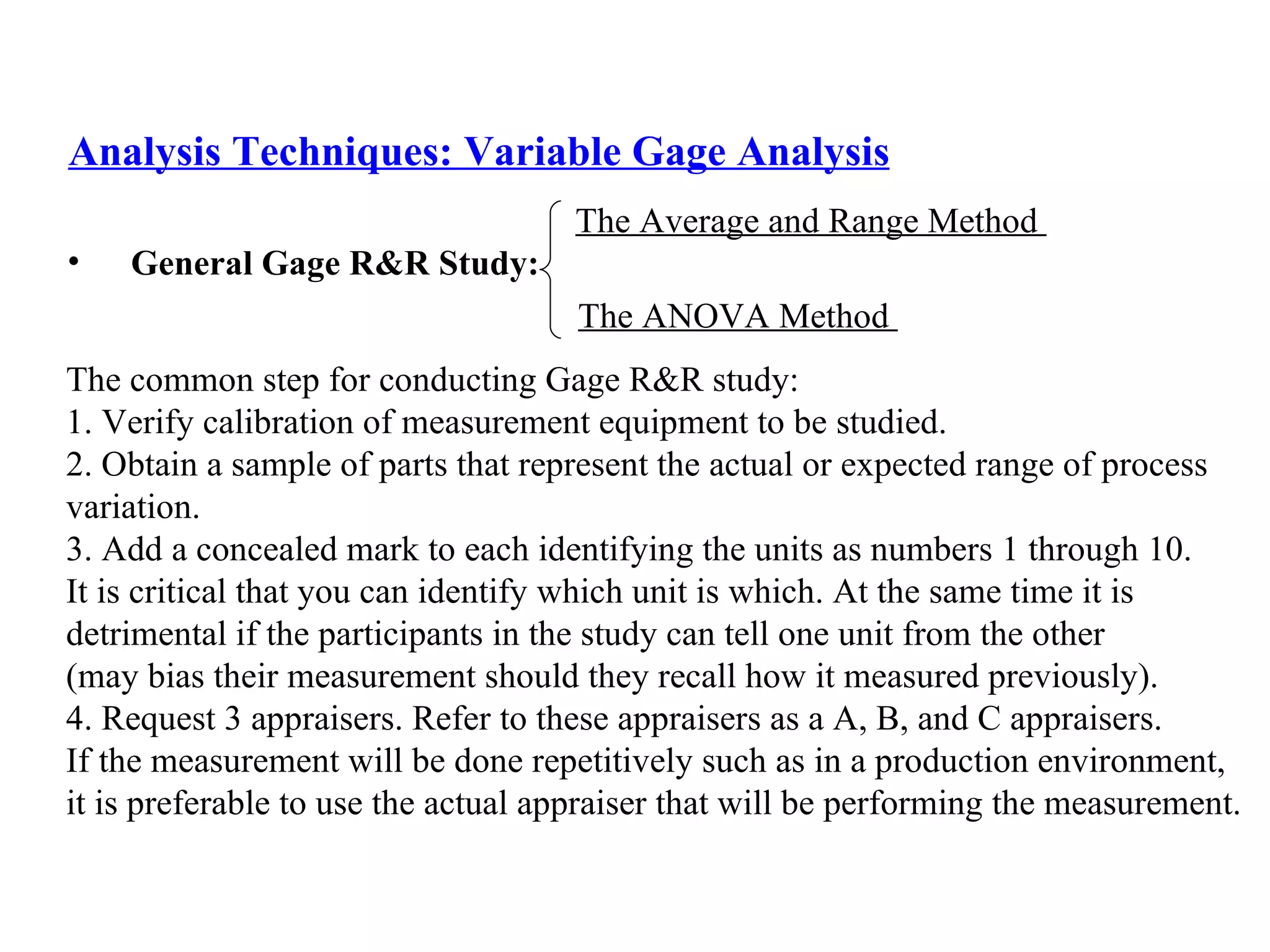
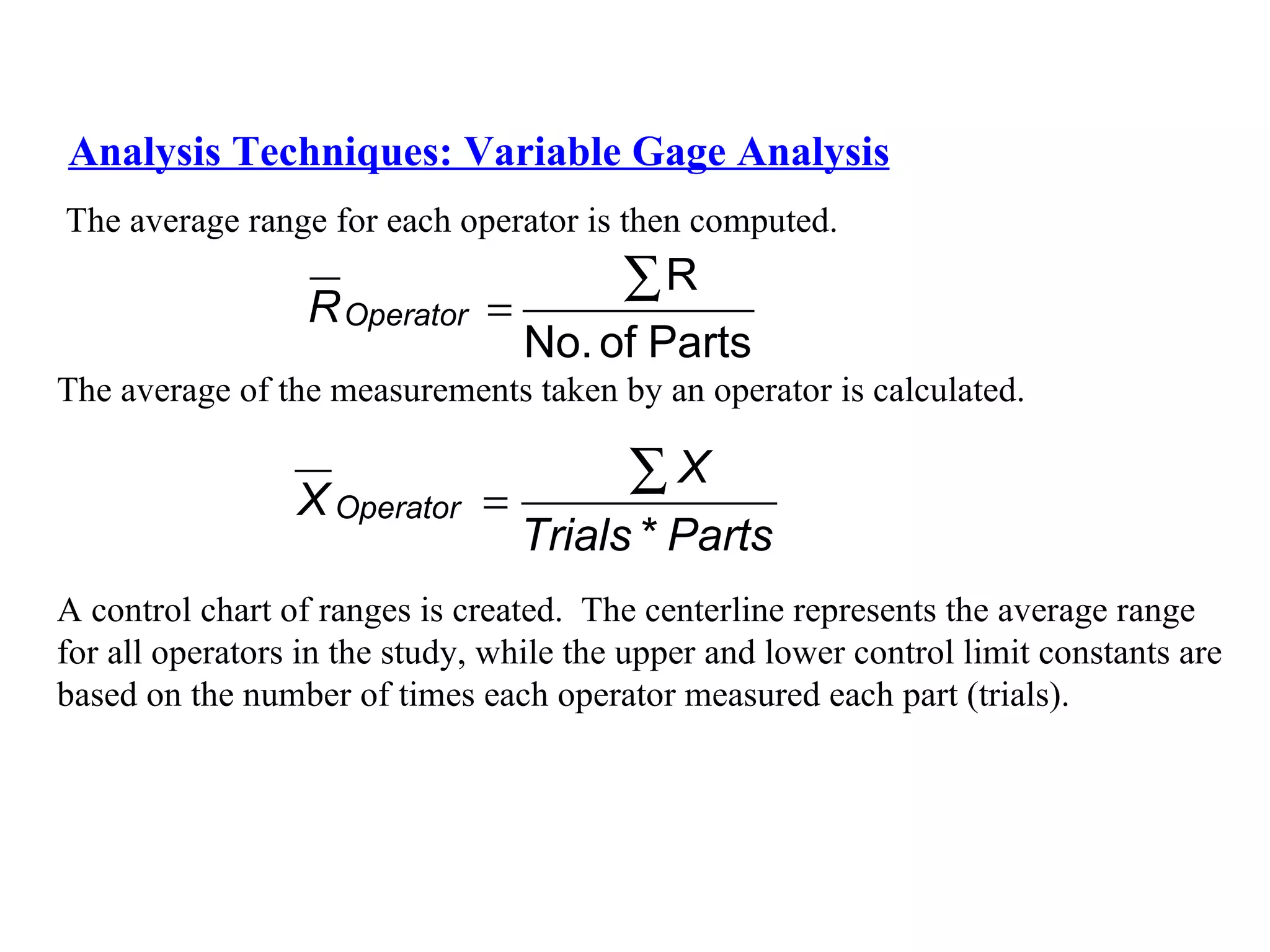
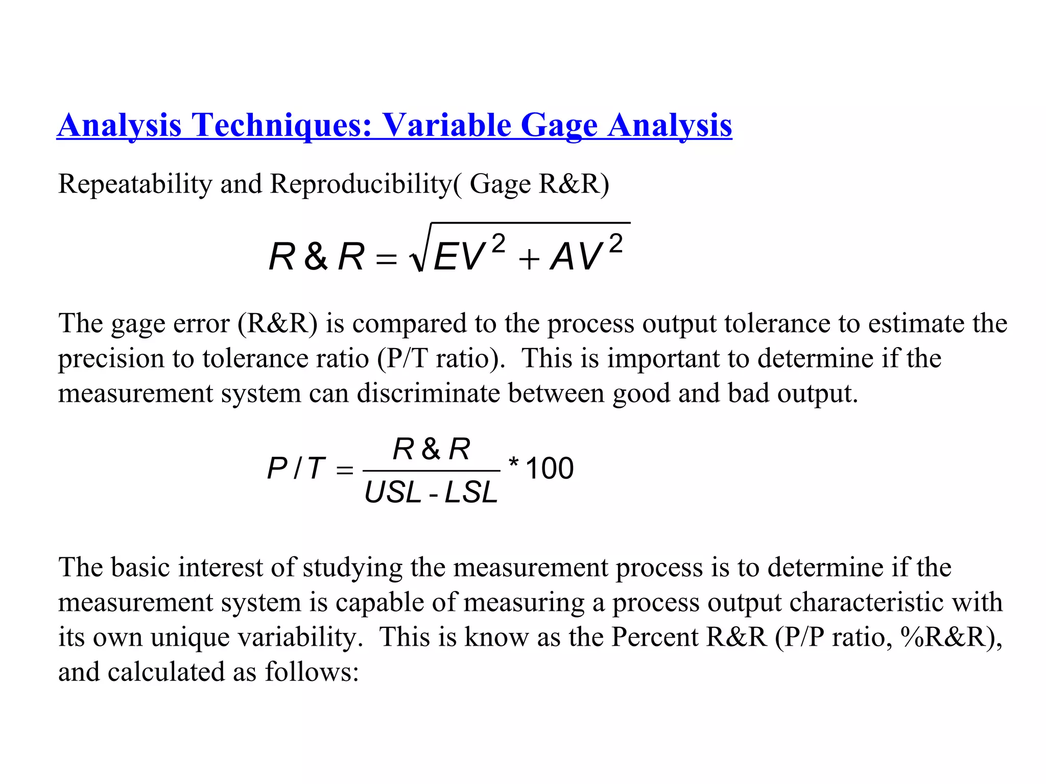
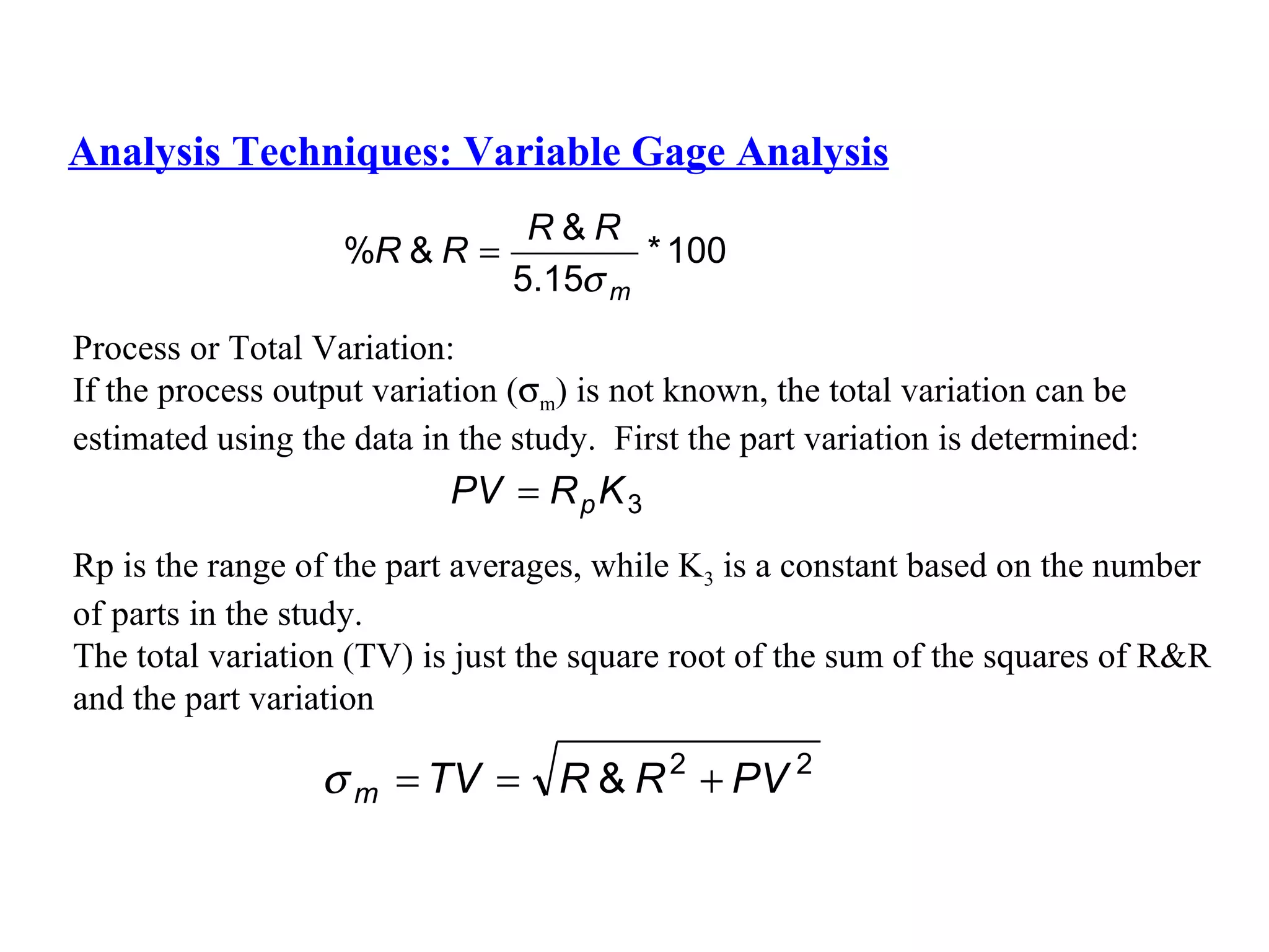
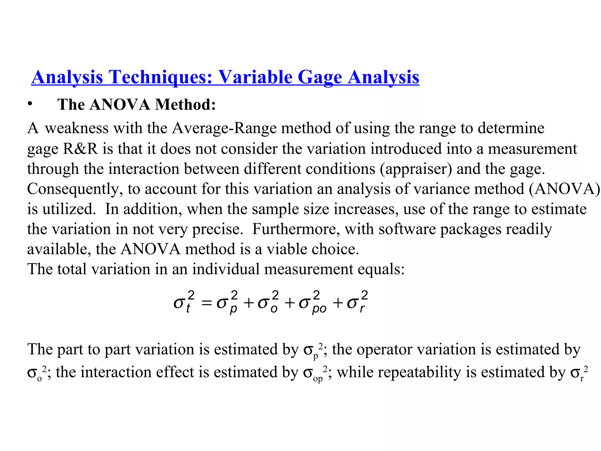
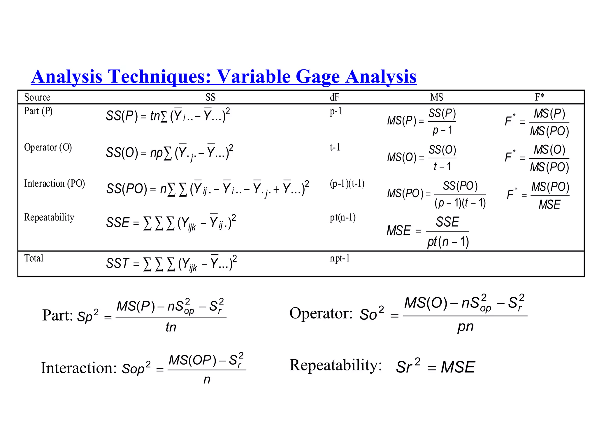
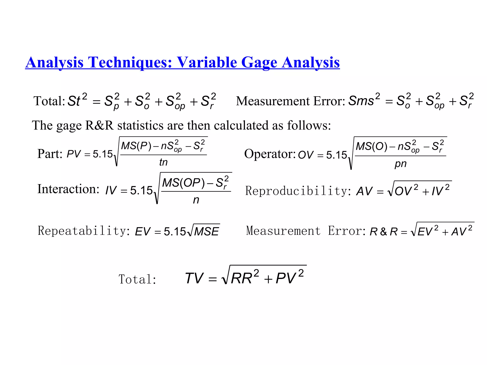
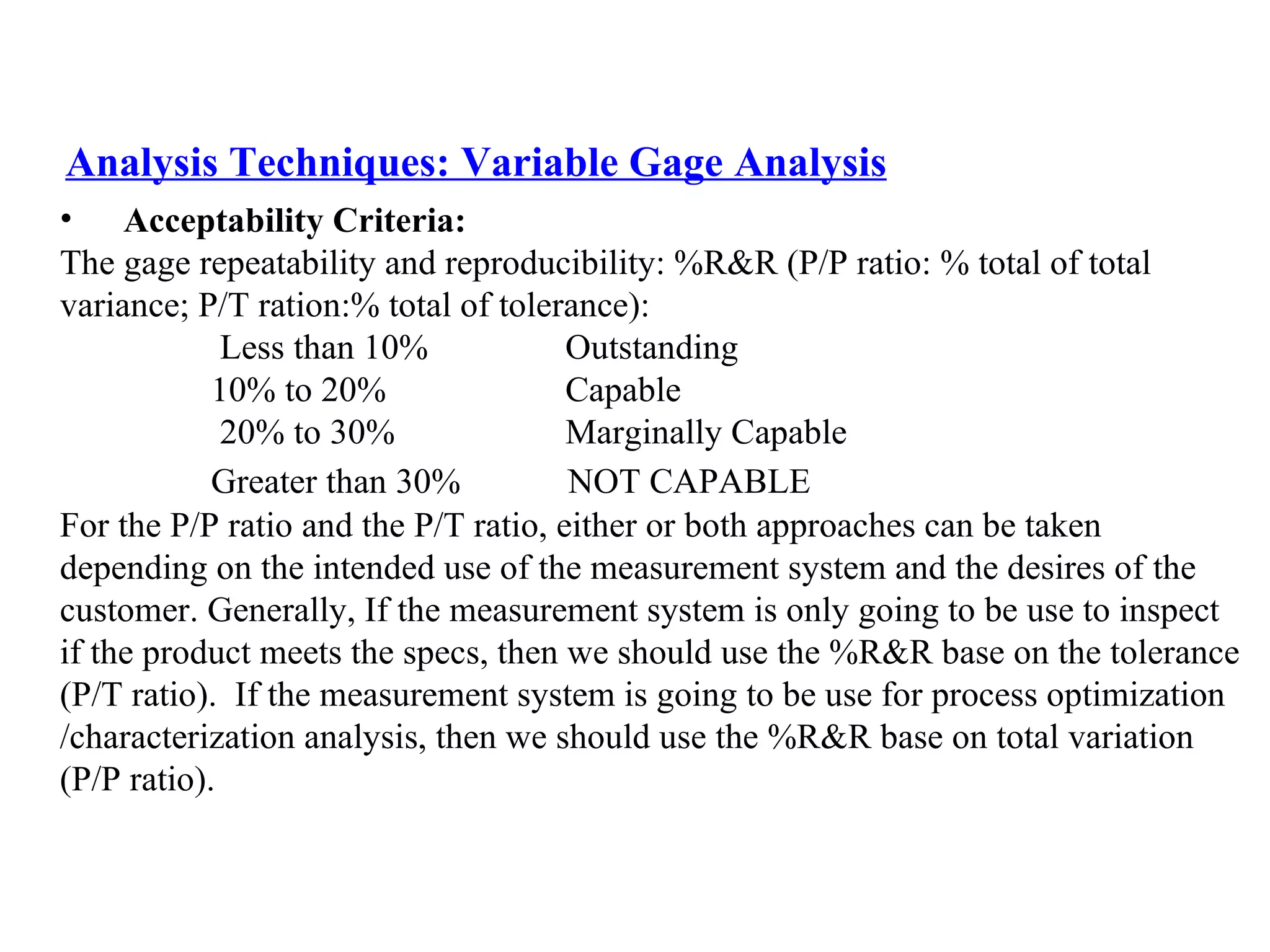
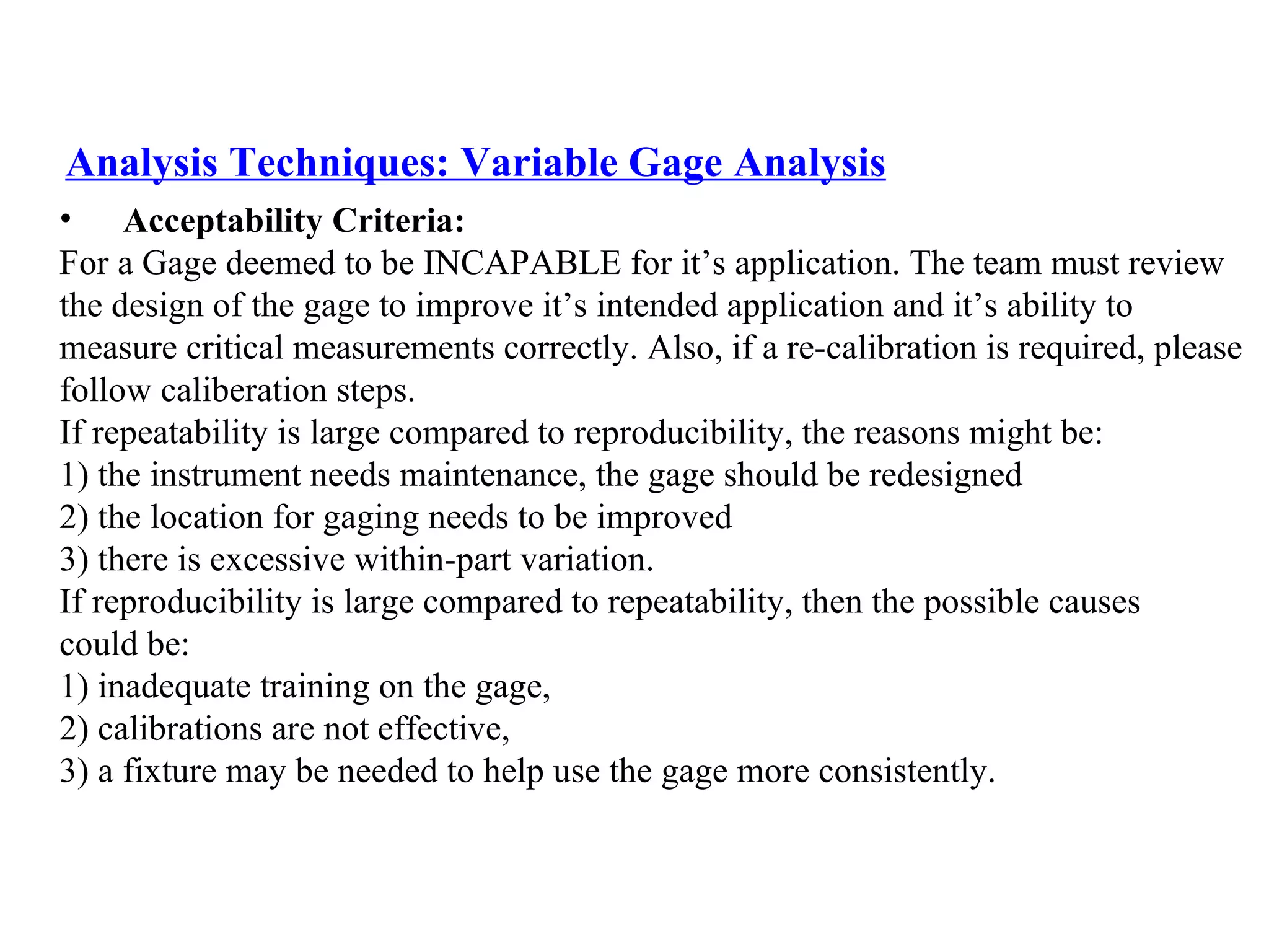
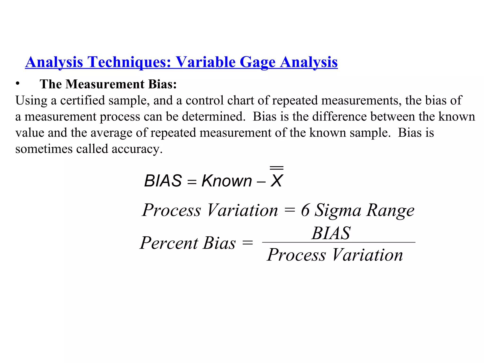
The document provides an overview of measurement system analysis (MSA) techniques for both variable and attribute gages. It describes the average-range method and ANOVA method for analyzing variable gages, and the short method, hypothesis test analysis, and long method for attribute gages. Acceptability criteria are outlined for determining if a measurement system is capable of measuring process variation.


![7 qc tools training material[1]](https://cdn.slidesharecdn.com/ss_thumbnails/7qctoolstrainingmaterial1-120925054558-phpapp02-thumbnail.jpg?width=640&height=640&fit=bounds)