Contents :
1) INTRODUCTIONFOR MEASUREMENT SYSTEM ANALYSIS
2) GENERAL METHODS ILLUSTRATION FOR
MEASUREMENT SYSTEM ANALYSIS
1) VARIABLE GAGE ANALYSIS METHOD
1) THE AVERAGE-RANGE METHOD
2) THE ANOVA METHOD
1) ATTRIBUTE GAGE ANALYSIS METHOD
1) SHORT METHOD
2) HYPOTHESIS TEST ANALYSIS
3) SIGNAL DETECTION THEORY
4) LONG METHOD
3) ACCEPTABILITY CRITERIA
4) CONCLUSION
5) FOUR METHODS COMPARISON
3.
Introduction: Basic requirementsby QS-9000 & TS16949
• Base on QS9000 & TS16949 requirements, all measurement system which were
mentioned in Quality Plan should be conducted Measurement System Analysis.
MSA
Requirement
4.
Introduction: The categoryof Measurement System
• Most industrial measurement system can be divided two categories, one is variable
measurement system, another is attribute measurement system. An attribute gage
cannot indicate how good or how bad a part is , but only indicates that the part is
accepted or rejected. The most common of these is a Go/No-go gage.
Variable Gage
Attribute Gage (Go/No-go Gage)
5.
Introduction: What isa measurement process
Operation Output
Input
General Process
Measurement Analysis
Value
Decision
Process to
be Managed
Measurement Process
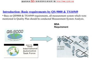
Measurement: The assignment of a numerical value to material things to represent the
relations among them with respect to a particular process.
Measurement Process: The process of assigning the numerical value to material things.
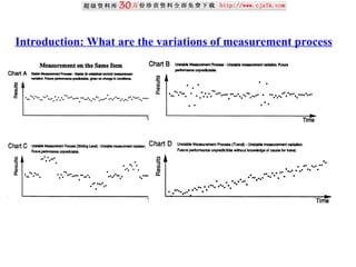
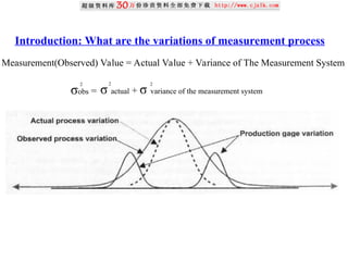
Introduction: What arethe variations of measurement process
Measurement(Observed) Value = Actual Value + Variance of The Measurement System
2
σobs =
2
σ actual + σ variance of the measurement system
2
8.
Introduction: Where doesthe variation of measurement system
come from?
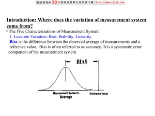
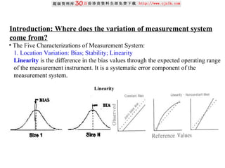
• The Five Characterizations of Measurement System:
1. Location Variation: Bias; Stability; Linearity
Bias is the difference between the observed average of measurements and a
reference value. Bias is often referred to as accuracy. It is a systematic error
component of the measurement system
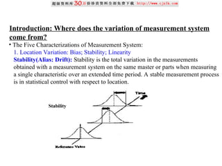
9.
Introduction: Where doesthe variation of measurement system
come from?
• The Five Characterizations of Measurement System:
1. Location Variation: Bias; Stability; Linearity
Stability(Alias: Drift): Stability is the total variation in the measurements
obtained with a measurement system on the same master or parts when measuring
a single characteristic over an extended time period. A stable measurement process
is in statistical control with respect to location.
Stability
10.
Introduction: Where doesthe variation of measurement system
come from?
• The Five Characterizations of Measurement System:
1. Location Variation: Bias; Stability; Linearity
Linearity is the difference in the bias values through the expected operating range
of the measurement instrument. It is a systematic error component of the
measurement system.
Linearity
11.
Introduction: Where doesthe variation of measurement system
come from?
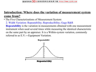
• The Five Characterizations of Measurement System:
2. Width Variation: Repeatability; Reproducibility; Gage R&R
Repeatability is the variation in measurements obtained with one measurement
instrument when used several times while measuring the identical characteristic
on the same part by an appraiser. It is a Within-system variation, commonly
referred to as E.V.---Equipment Variation.
Repeatability
12.
Introduction: Where doesthe variation of measurement system
come from?
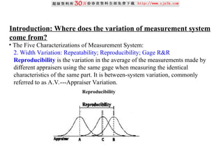
• The Five Characterizations of Measurement System:
2. Width Variation: Repeatability; Reproducibility; Gage R&R
Reproducibility is the variation in the average of the measurements made by
different appraisers using the same gage when measuring the identical
characteristics of the same part. It is between-system variation, commonly
referred to as A.V.---Appraiser Variation.
Reproducibility
13.
Introduction: Where doesthe variation of measurement system
come from?
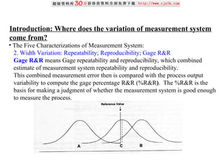
• The Five Characterizations of Measurement System:
2. Width Variation: Repeatability; Reproducibility; Gage R&R
Gage R&R means Gage repeatability and reproducibility, which combined
estimate of measurement system repeatability and reproducibility.
This combined measurement error then is compared with the process output
variability to compute the gage percentage R&R (%R&R). The %R&R is the
basis for making a judgment of whether the measurement system is good enough
to measure the process.
14.
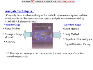
Analysis Techniques:
• Currentlythere are three techniques for variable measurement system and four
techniques for attribute measurement system analysis were recommended by
AIAG MSA Reference Manual.
• Range Method
• Average - Range
Method
• ANOVA
• Short Method
• Long Method
• Hypothesis Test Analyses
• Signal Detection Theory
• Followings are some practical examples to illustrate how to perform four
methods respectively.
Variable Gage Attribute Gage
15.
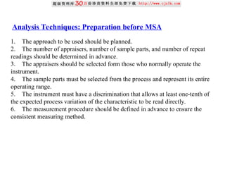
Analysis Techniques: Preparationbefore MSA
1. The approach to be used should be planned.
2. The number of appraisers, number of sample parts, and number of repeat
readings should be determined in advance.
3. The appraisers should be selected form those who normally operate the
instrument.
4. The sample parts must be selected from the process and represent its entire
operating range.
5. The instrument must have a discrimination that allows at least one-tenth of
the expected process variation of the characteristic to be read directly.
6. The measurement procedure should be defined in advance to ensure the
consistent measuring method.
16.
Analysis Techniques: VariableGage Analysis
1. General Gage R&R Study:
The Average and Range Method
The ANOVA Method
The common step for conducting Gage R&R study:
1. Verify calibration of measurement equipment to be studied.
2. Obtain a sample of parts that represent the actual or expected range of process
variation.
3. Add a concealed mark to each identifying the units as numbers 1 through 10.
It is critical that you can identify which unit is which. At the same time it is
detrimental if the participants in the study can tell one unit from the other
(may bias their measurement should they recall how it measured previously).
4. Request 3 appraisers. Refer to these appraisers as a A, B, and C appraisers.
If the measurement will be done repetitively such as in a production environment,
it is preferable to use the actual appraiser that will be performing the measurement.
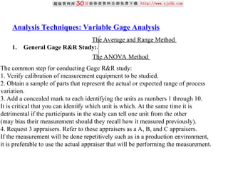
17.
For extreme cases,a minimum of two appraisers can be used, but this is strongly
discouraged as a less accurate estimate of measurement variation will result.
5. Let appraiser A measure 10 parts in a random order while you record the data
noting the concealed marking. Let appraisers B and C measure the same 10 parts
Note: Do not allow the appraisers to witness each other performing the
measurement. The reason is the same as why the unit markings are concealed,
TO PREVENT BIAS.
6. Repeat the measurements for all three appraisers, but this time present the
samples to each in a random order different from the original measurements.
This is to again help reduce bias in the measurements.
Analysis Techniques: Variable Gage Analysis
……
10 Parts 3 Appraisers
3 Trials
18.
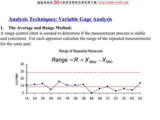
1. The Averageand Range Method:
A range control chart is created to determine if the measurement process is stable
and consistent. For each appraiser calculate the range of the repeated measurements
for the same part.
Analysis Techniques: Variable Gage Analysis
Range of Repeated Measures
0
10
20
30
40
1A 2A 3A 4A 5A 1B 2B 3B 4B 5B 1C 2C 3C 4C 5C
0.01M
M
Min
X
X
R
Range Max -
19.
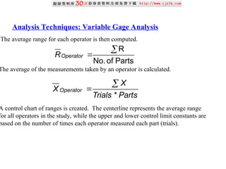
Analysis Techniques: VariableGage Analysis
The average range for each operator is then computed.
The average of the measurements taken by an operator is calculated.
A control chart of ranges is created. The centerline represents the average range
for all operators in the study, while the upper and lower control limit constants are
based on the number of times each operator measured each part (trials).
Parts
of
No.
R
Operator
R
Parts
Trials
X
X Operator
*
20.
Analysis Techniques: VariableGage Analysis
R
D
LCL
R
D
UCL
R
R
R
R
3
4
Operators
No.of
The centerline and control limits are graphed onto a control chart and the
calculated ranges are then plotted on the control chart. The range control chart is
examined to determine measurement process stability. If any of the plotted ranges
fall outside the control limits the measurement process is not stable, and further
analysis should not take place. However, it is common to have the particular
operator re-measure the particular process output again and use that data if it is
in-control.
21.
Analysis Techniques: VariableGage Analysis
Repeatability - Equipment Variation (E.V.)
The constant d2
*
is based on the number of measurements used to compute the
individual ranges(n) or trials, the number of parts in the study, and the number of
different conditions under study. The constant K1 is based on the number of times
a part was repeatedly measured (trials).
The equipment variation is often compared to the process output tolerance or
process output variation to determine a percent equipment variation (%EV).
1
2
*
*
15
.
5 K
R
d
R
EV
100
*
15
.
5
)
(
%
100
*
)
(
%
m
EV
PROC
EV
LSL
USL
EV
TOL
EV
22.
Analysis Techniques: VariableGage Analysis
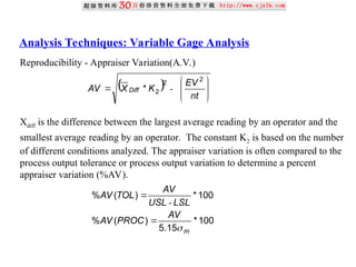
Reproducibility - Appraiser Variation(A.V.)
Xdiff is the difference between the largest average reading by an operator and the
smallest average reading by an operator. The constant K2 is based on the number
of different conditions analyzed. The appraiser variation is often compared to the
process output tolerance or process output variation to determine a percent
appraiser variation (%AV).
nt
EV
K
X
AV Diff
2
2
2
* -
100
*
15
.
5
)
(
%
100
*
)
(
%
m
AV
PROC
AV
LSL
USL
AV
TOL
AV
-
23.
Analysis Techniques: VariableGage Analysis
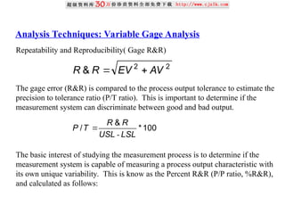
Repeatability and Reproducibility( Gage R&R)
The gage error (R&R) is compared to the process output tolerance to estimate the
precision to tolerance ratio (P/T ratio). This is important to determine if the
measurement system can discriminate between good and bad output.
The basic interest of studying the measurement process is to determine if the
measurement system is capable of measuring a process output characteristic with
its own unique variability. This is know as the Percent R&R (P/P ratio, %R&R),
and calculated as follows:
2
2
& AV
EV
R
R
100
*
&
/
LSL
USL
R
R
T
P
-
24.
Analysis Techniques: VariableGage Analysis
100
*
15
.
5
&
&
%
m
R
R
R
R
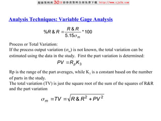
Process or Total Variation:
If the process output variation (m) is not known, the total variation can be
estimated using the data in the study. First the part variation is determined:
Rp is the range of the part averages, while K3 is a constant based on the number
of parts in the study.
The total variation (TV) is just the square root of the sum of the squares of R&R
and the part variation
3
K
R
PV p
2
2
& PV
R
R
TV
m
25.
Analysis Techniques: VariableGage Analysis
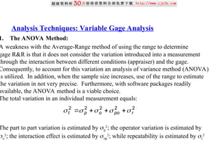
1. The ANOVA Method:
A weakness with the Average-Range method of using the range to determine
gage R&R is that it does not consider the variation introduced into a measurement
through the interaction between different conditions (appraiser) and the gage.
Consequently, to account for this variation an analysis of variance method (ANOVA)
is utilized. In addition, when the sample size increases, use of the range to estimate
the variation in not very precise. Furthermore, with software packages readily
available, the ANOVA method is a viable choice.
The total variation in an individual measurement equals:
The part to part variation is estimated by p
2
; the operator variation is estimated by
o
2
; the interaction effect is estimated by op
2
; while repeatability is estimated by r
2
2
2
2
2
2
r
po
o
p
t
26.
Analysis Techniques: VariableGage Analysis
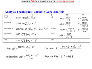
Source SS dF MS F*
Part (P)
2
...)
..
(
)
( Y
Y
tn
P
SS i
p-1
1
)
(
)
(
p
P
SS
P
MS
)
(
)
(
*
PO
MS
P
MS
F
Operator (O)
2
...)
.
.
(
)
( Y
Y
np
O
SS j
t-1
1
)
(
)
(
t
O
SS
O
MS
)
(
)
(
*
PO
MS
O
MS
F
Interaction (PO)
2
...)
.
.
..
.
(
)
( Y
Y
Y
Y
n
PO
SS j
i
ij
(p-1)(t-1)
)
1
)(
1
(
)
(
)
(
t
p
PO
SS
PO
MS
MSE
PO
MS
F
)
(
*
Repeatability
2
.)
( ij
ijk Y
Y
SSE pt(n-1)
)
1
(
n
pt
SSE
MSE
Total
2
...)
( Y
Y
SST ijk
npt-1
Part:
tn
S
nS
P
MS
Sp
r
op
2
2
2
)
(
Operator:
pn
S
nS
O
MS
So
r
op
2
2
2
)
(
Interaction:
n
S
OP
MS
Sop r
2
2 )
(
Repeatability: MSE
Sr
2
27.
Analysis Techniques: VariableGage Analysis
Total: 2
2
2
2
2
r
op
o
p S
S
S
S
St
The gage R&R statistics are then calculated as follows:
2
2
2
2
r
op
o S
S
S
Sms
Measurement Error:
Part:
tn
S
nS
P
MS
PV
r
op
2
2
)
(
15
.
5
Operator:
pn
S
nS
O
MS
OV
r
op
2
2
)
(
15
.
5
Interaction:
n
S
OP
MS
IV r
2
)
(
15
.
5
Reproducibility: 2
2
IV
OV
AV
Repeatability: MSE
EV 15
.
5
Measurement Error: 2
2
& AV
EV
R
R
Total:
2
2
PV
RR
TV
28.
Analysis Techniques: VariableGage Analysis
1. Acceptability Criteria:
The gage repeatability and reproducibility: %R&R (P/P ratio: % total of total
variance; P/T ration:% total of tolerance):
Less than 10% Outstanding
10% to 20% Capable
20% to 30% Marginally Capable
Greater than 30% NOT CAPABLE
For the P/P ratio and the P/T ratio, either or both approaches can be taken
depending on the intended use of the measurement system and the desires of the
customer. Generally, If the measurement system is only going to be use to inspect
if the product meets the specs, then we should use the %R&R base on the tolerance
(P/T ratio). If the measurement system is going to be use for process optimization
/characterization analysis, then we should use the %R&R base on total variation
(P/P ratio).
29.
Analysis Techniques: VariableGage Analysis
1. Acceptability Criteria:
For a Gage deemed to be INCAPABLE for it’s application. The team must review
the design of the gage to improve it’s intended application and it’s ability to
measure critical measurements correctly. Also, if a re-calibration is required, please
follow caliberation steps.
If repeatability is large compared to reproducibility, the reasons might be:
1) the instrument needs maintenance, the gage should be redesigned
2) the location for gaging needs to be improved
3) there is excessive within-part variation.
If reproducibility is large compared to repeatability, then the possible causes
could be:
1) inadequate training on the gage,
2) calibrations are not effective,
3) a fixture may be needed to help use the gage more consistently.
30.
Analysis Techniques: VariableGage Analysis
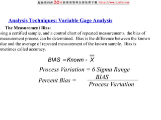
. The Measurement Bias:
Using a certified sample, and a control chart of repeated measurements, the bias of
measurement process can be determined. Bias is the difference between the known
alue and the average of repeated measurement of the known sample. Bias is
ometimes called accuracy.
X
Known
BIAS
Process Variation = 6 Sigma Range
Percent Bias =
BIAS
Process Variation
31.
Analysis Techniques: VariableGage Analysis
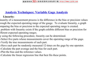
. Linearity:
inearity of a measurement process is the difference in the bias or precision values
hrough the expected operating range of the gauge. To evaluate linearity, a graph
omparing the bias or precision to the expected operating range is created.
A problem with linearity exists if the graph exhibits different bias or precision for
ifferent expected operating ranges.
y using the following procedure, linearity can be determined.
) Select five parts whose measurements cover the operating range of the gage.
) Verify the true measurements of each part.
) Have each part be randomly measured 12 times on the gage by one operator.
) Calculate the part average and the bias for each part.
) Plot the bias and the reference values.
) Calculate the linear regression line that best fits these points.
32.
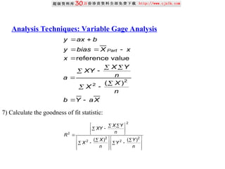
Analysis Techniques: VariableGage Analysis
X
a
Y
b
n
X
X
n
Y
X
XY
a
x
x
X
bias
y
b
ax
y
Part
2
2 )
(
value
reference
7) Calculate the goodness of fit statistic:
n
Y
Y
n
X
X
n
Y
X
XY
R
2
2
2
2
2
2
)
(
)
(
33.
Analysis Techniques: VariableGage Analysis
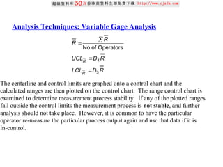
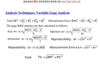
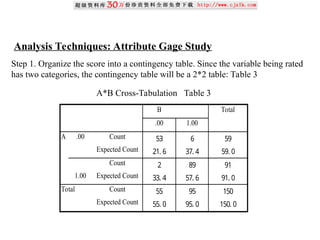
8) Determine linearity and percent linearity:
Linearity = Slope x Process variation(m)
%Linearity = 100[linearity/Process Variation]
The acceptability criteria of Bias, Linearity depend on Quality Control Plan,
characteristic being measured and gage speciality, suggested criteria of ESG is
as following:
Under 5% - acceptable
5% to 15% - may be acceptable based upon importance of application, cost of
measurement device, cost of repairs, etc.,
Over 15% - Considered not acceptable - every effort should be made to improve
the system
The stability is determined through the use of a control chart. It is important to
note that, when using control charts, one must not only watch for points that fall
outside of the control limits, but also care other special cause signals such as trends
and centerline hugging.Guideline for the detection of such signals can be found in
many publications on SPC.
34.
Analysis Techniques: AttributeGage Study
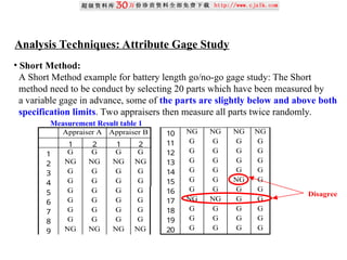
• Short Method:
A Short Method example for battery length go/no-go gage study: The Short
method need to be conduct by selecting 20 parts which have been measured by
a variable gage in advance, some of the parts are slightly below and above both
specification limits. Two appraisers then measure all parts twice randomly.
Appraiser A Appraiser B
1 2 1 2
1 G G G G
2 NG NG NG NG
3 G G G G
4 G G G G
5 G G G G
6 G G G G
7 G G G G
8 G G G G
9 NG NG NG NG
10 NG NG NG NG
11 G G G G
12 G G G G
13 G G G G
14 G G G G
15 G G NG G
16 G G G G
17 NG NG G G
18 G G G G
19 G G G G
20 G G G G
Disagree
Measurement Result table 1
35.
Analysis Techniques: AttributeGage Study
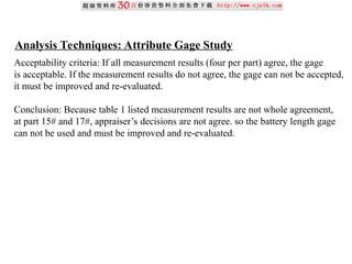
Acceptability criteria: If all measurement results (four per part) agree, the gage
is acceptable. If the measurement results do not agree, the gage can not be accepted,
it must be improved and re-evaluated.
Conclusion: Because table 1 listed measurement results are not whole agreement,
at part 15# and 17#, appraiser’s decisions are not agree. so the battery length gage
can not be used and must be improved and re-evaluated.
36.
Analysis Techniques: AttributeGage Study
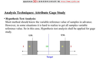
• Hypothesis Test Analysis:
Short method should know the variable reference value of samples in advance.
However, in some situations it is hard to realize to get all samples variable
reference value. So in this case, Hypothesis test analysis shall be applied for gage
study.
II
II
Target
I
I III
USL
LSL
37.
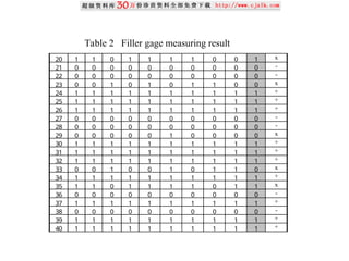
Analysis Techniques: AttributeGage Study
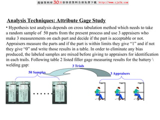
• Hypothesis test analysis depends on cross tabulation method which needs to take
a random sample of 50 parts from the present process and use 3 appraisers who
make 3 measurements on each part and decide if the part is acceptable or not.
Appraisers measure the parts and if the part is within limits they give “1” and if not
they give “0” and write those results in a table. In order to eliminate any bias
produced, the labeled samples are mixed before giving to appraisers for identification
in each trails. Following table 2 listed filler gage measuring results for the battery
welding gap:
……
50 Samples 3 Appraisers
3 Trials
41 0 00 0 0 0 0 0 0 0 -
42 1 0 1 1 1 1 1 1 0 1 x
43 1 1 1 1 1 1 1 1 1 1 +
44 1 1 1 1 1 1 1 1 1 1 +
45 1 1 1 1 1 1 1 1 1 1 +
46 0 0 0 0 0 0 0 0 0 0 -
47 0 0 0 0 0 0 0 0 0 0 -
48 1 1 1 1 1 1 1 1 1 1 +
49 0 0 0 0 0 0 0 0 0 0 -
50 1 1 1 1 1 1 1 1 1 1 +
Table 2 Filler gage measuring result
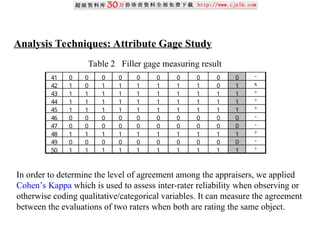
Analysis Techniques: Attribute Gage Study
In order to determine the level of agreement among the appraisers, we applied
Cohen’s Kappa which is used to assess inter-rater reliability when observing or
otherwise coding qualitative/categorical variables. It can measure the agreement
between the evaluations of two raters when both are rating the same object.
41.
Step 1. Organizethe score into a contingency table. Since the variable being rated
has two categories, the contingency table will be a 2*2 table: Table 3
Analysis Techniques: Attribute Gage Study
B Total
.00 1.00
A .00 Count 53 6 59
Expected Count 21. 6 37. 4 59. 0
Count 2 89 91
1.00 Expected Count 33. 4 57. 6 91. 0
Total Count 55 95 150
Expected Count 55. 0 95. 0 150. 0
A*B Cross-Tabulation Table 3
42.
Analysis Techniques: AttributeGage Study
Step 2. Compute the row totals (sum across the values on the same row) and
column totals of the observed frequencies.
Step 3 Compute the overall total (show in the table 3). As a computational check,
be sure that the row totals and the column totals sum to the same value for the
overall total, and the overall total matches the number of cases in the original data set.
Step 4 Compute the total number of agreements by summing the values in the
diagonal cells of the table.
Σa = 53+ 89 = 142
Step 5 Compute the expected frequency for the number of agreements that would
have been expected by chance for each coding category.
ef = = = 21.6
Repeat the formula for other cell, we got other expected count (show in the table 3).
row total * col total
overall total
59 * 55
150
43.
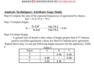
Step 6 Computethe sum of the expected frequencies of agreement by chance.
Σef = 21.6+57.6 = 79.2
Step 7 Compute Kappa
K = = = 0.89
Step 8 Evaluate Kappa
- A general rule of thumb is that values of kappa greater than 0.75 indicate
good to excellent agreement; values less than 0.4 indicate poor agreement.
Repeat above step, we can got following kappa measures for the appraisers: Table
4
Analysis Techniques: Attribute Gage Study
Σa-Σef
N-Σef
142-79.2
150-79.2
Kappa A B C
A - 0. 89 0. 83
B 0. 89 - 0. 85
C 0. 83 0. 85 -
Table 4
44.
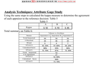
Using the samesteps to calculated the kappa measure to determine the agreement
of each appraiser to the reference decision: Table 5
Total summary on Table 6:
Analysis Techniques: Attribute Gage Study
A B C
Kappa 0. 92 0. 93 0. 85
Table 5
Source Appraiser A Appraiser B Appraiser C
Total Inspected 50 50 50
# Matched 44 46 43
Mixed 6 4 7
95%UCI 95. 50% 97. 80% 94. 20%
Calculated Score 88% 92% 86%
95%LCI 75. 70% 81% 73. 30%
Total Inspected 50
# in Agreement 42
95%UCI 92. 80%
Calculated Score 84%
95%LCI 73. 70%
%Score vs Attribute
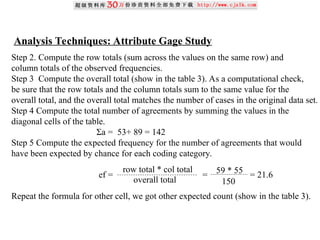
45.
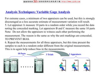
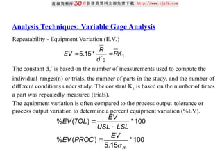
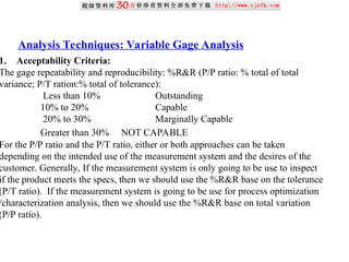
Anne Ben Cathy
75
85
95
Appraiser
Percent
WithinAppraiser
Anne Ben Cathy
75
85
95
Appraiser
Percent
Appraiser vs Standard
Assessment Agreement
Date of study:
Reported by:
Name of product:
Misc:
[ , ] 95.0% CI
Percent
Analysis Techniques: Attribute Gage Study
46.
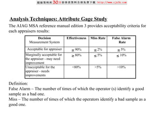
Analysis Techniques: AttributeGage Study
The AIAG MSA reference manual edition 3 provides acceptability criteria for
each appraisers results:
Definition:
False Alarm – The number of times of which the operator (s) identify a good
sample as a bad one.
Miss – The number of times of which the operators identify a bad sample as a
good one.
Decision
Measurement System
Effectiveness Miss Rate False Alarm
Rate
Acceptable for appraiser ≥ 90% ≤ 2% ≤ 5%
Marginally acceptable for
the appraiser - may need
improvement
≥ 80% ≤ 5% ≤ 10%
Unacceptable for the
appraiser - needs
improvements
<80% >5% >10%
47.
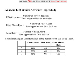
Number of correctdecisions
Total opportunities for a decision
Effectiveness =
Analysis Techniques: Attribute Gage Study
Number of False Alarm
Total opportunities for a decision
False Alarm Rate =
Number of False Alarm
Total opportunities for a decision
Miss Rate =
So summarizing all the information of the example with this table: Table 7
False Alarm
Rate
A 88% 4% 8%
B 92% 6% 2%
C 86% 8% 14%
Effectiveness Miss Rate
48.
Analysis Techniques: AttributeGage Study
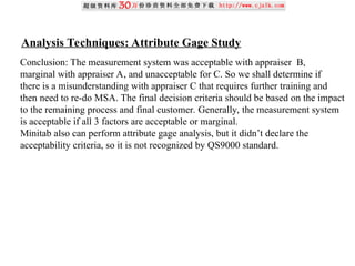
Conclusion: The measurement system was acceptable with appraiser B,
marginal with appraiser A, and unacceptable for C. So we shall determine if
there is a misunderstanding with appraiser C that requires further training and
then need to re-do MSA. The final decision criteria should be based on the impact
to the remaining process and final customer. Generally, the measurement system
is acceptable if all 3 factors are acceptable or marginal.
Minitab also can perform attribute gage analysis, but it didn’t declare the
acceptability criteria, so it is not recognized by QS9000 standard.
49.
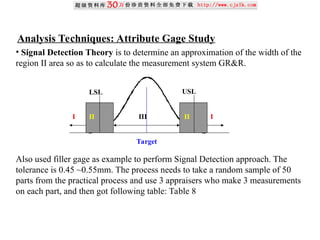
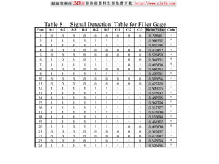
Analysis Techniques: AttributeGage Study
• Signal Detection Theory is to determine an approximation of the width of the
region II area so as to calculate the measurement system GR&R.
Also used filler gage as example to perform Signal Detection approach. The
tolerance is 0.45 ~0.55mm. The process needs to take a random sample of 50
parts from the practical process and use 3 appraisers who make 3 measurements
on each part, and then got following table: Table 8
II
II
Target
I
I III
USL
LSL
Analysis Techniques: AttributeGage Study
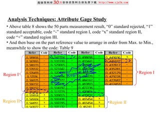
• Above table 8 shows the 50 parts measurement result, “0” standard rejected, “1”
standard acceptable, code “-” standard region I, code “x” standard region II,
code “+” standard region III.
• And then base on the part reference value to arrange in order from Max. to Min.,
meanwhile to show the code: Table 9
Refer Code
0. 589656 -
0. 587893 -
0. 580273 -
0. 576532 -
0. 576459 -
0. 57036 -
0. 566575 -
0. 566152 -
0. 566152 -
0. 561457 -
0. 559918 x
0. 545604 x
0. 544951 x
0. 543077 x
Refer Code
0. 542704 +
0. 531939 +
0. 529065 +
0. 521642 +
0. 520496 +
0. 519694 +
0. 517377 +
0. 515537 +
0. 514192 +
0. 513779 +
0. 509015 +
0. 502436 +
0. 502295 +
0. 501132 +
Refer Code
0. 498698 +
0. 493441 +
0. 488905 +
0. 488184 +
0. 487613 +
0. 486379 +
0. 484167 +
0. 483803 +
0. 477236 +
0. 476901 +
0. 470832 +
0. 465454 x
0. 465454 x
0. 46241 x
Refer Code
0. 449696 x
0. 446697 -
0. 437817 -
0. 435281 -
0. 432179 -
0. 429228 -
0. 427687 -
0. 412453 -
Region III Region I
Region I
Region II Region II
53.
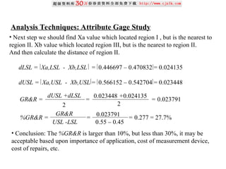
Analysis Techniques: AttributeGage Study
• Next step we should find Xa value which located region I , but is the nearest to
region II. Xb value which located region III, but is the nearest to region II.
And then calculate the distance of region II.
dLSL = Xa,LSL - Xb,LSL = 0.446697 – 0.470832 = 0.024135
dUSL = Xa,USL - Xb,USL = 0.566152 – 0.542704 = 0.023448
0.023791
0.55 – 0.45
GR&R = = = 0.023791
dUSL +dLSL
2
0.023448 +0.024135
2
%GR&R = = = 0.277 = 27.7%
GR&R
USL -LSL
• Conclusion: The %GR&R is larger than 10%, but less than 30%, it may be
acceptable based upon importance of application, cost of measurement device,
cost of repairs, etc.
54.
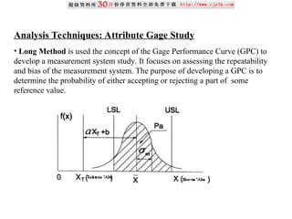
Analysis Techniques: AttributeGage Study
• Long Method is used the concept of the Gage Performance Curve (GPC) to
develop a measurement system study. It focuses on assessing the repeatability
and bias of the measurement system. The purpose of developing a GPC is to
determine the probability of either accepting or rejecting a part of some
reference value.
55.
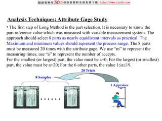
• The firststep of Long Method is the part selection. It is necessary to know the
part reference value which was measured with variable measurement system. The
approach should select 8 parts as nearly equidistant intervals as practical. The
Maximum and minimum values should represent the process range. The 8 parts
must be measured 20 times with the attribute gage. We use “m” to represent the
measuring times, use “a” to represent the number of accepts.
For the smallest (or largest) part, the value must be a=0; For the largest (or smallest)
part, the value must be a=20; For the 6 other parts, the value 1≤a≤19.
Analysis Techniques: Attribute Gage Study
……
8 Samples
1 Appraiser
20 Trials
56.
Analysis Techniques: AttributeGage Study
Reference
Value (Actual
Measurement)
(XT)
Number of
Accepts (a)
0.26 0
0.25 1
0.24 2
0.23 5
0.22 9
0.21 15
0.2 20
0.17 20
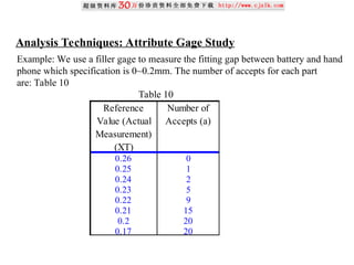
Example: We use a filler gage to measure the fitting gap between battery and hand
phone which specification is 0~0.2mm. The number of accepts for each part
are: Table 10
Table 10
57.
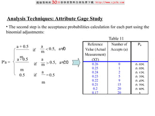
Analysis Techniques: AttributeGage Study
• The second step is the acceptance probabilities calculation for each part using the
binomial adjustments:
Reference
Value (Actual
Measurement)
(XT)
Number of
Accepts (a)
Pa
0.26 0 0. 025
0.25 1 0. 075
0.24 2 0. 125
0.23 5 0. 275
0.22 9 0. 475
0.21 15 0. 725
0.2 20 0. 975
0.17 20 1
Table 11
P'a =
<
if
a + 0.5
m
a
m
0.5, a≠0
>
if
a - 0.5
m
a
m 0.5, a≠20
0.5 if
a
m
0.5
=
58.
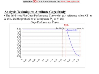
Analysis Techniques: AttributeGage Study
• The third step: Plot Gage Performance Curve with part reference value XT as
X axis, and the probability of acceptance P'a
as Y axis
Gage Performance Curve
0
0. 05
0. 1
0. 15
0. 2
0. 25
0. 3
0. 35
0. 4
0. 45
0. 5
0. 55
0. 6
0. 65
0. 7
0. 75
0. 8
0. 85
0. 9
0. 95
1
1. 05
USL
Repeatability
Pa=0.5%
Pa=99.5%
59.
Analysis Techniques: AttributeGage Study
• The fourth step: Base on Gage Performance Curve to find XT value at Pa
= 0.5%
and Pa
= 99.5% (using normal probability paper can get more accurate estimates).
We also can use Statistical Forecast calculation to get the XT value.
XT = 0.264 at Pa
= 0.5% XT = 0.184 at Pa
= 99.5%
Bias = XT (at Pa
= 0.5%)-USL = 0.264 – 0.2 =0.064
The repeatability is determined by finding the differences of the XT value
corresponding to Pa
= 99.5% and Pa
= 0.05% and dividing by an adjustment factor
of 1.08. Repeatability =
XT(at Pa = 0.5%) - XT(at Pa = 99.5%)
1.08
= = 0.074
0.264 – 0.184
1.08
60.
Analysis Techniques: AttributeGage Study
• Conclusion: Because the filler gage repeatability is 7.4% , Bias is 6.4%. Both of
them are less than 10%, so the gage can be accepted to use.
61.
Four Methods Comparison
•The four methods for attribute measurement study have respective feature. The
Short method look like simple, but it need to select enough parts which are slightly
below and above both specification limits, and must measure variable reference
value in advance. Hypothesis Test didn’t need to measure the variable reference
value, so it is feasible for manufacturing, but it need large sample size. Signal
Detection method can determine an approximation of the width of the region II
area so as to calculate the measurement system GR&R. Long method is used the
concept of the Gage Performance Curve (GPC) to assess the repeatability and bias
of the measurement system. When the importance of the measurement system
need to be highly assured, the Signal Detection method and Long method would
be necessary. Although the statistical calculation process for above methods is
complex, now we are designing a software to be able to perform the four methods
process and calculation.


![Analysis Techniques: Variable Gage Analysis
8) Determine linearity and percent linearity:
Linearity = Slope x Process variation(m)
%Linearity = 100[linearity/Process Variation]
The acceptability criteria of Bias, Linearity depend on Quality Control Plan,
characteristic being measured and gage speciality, suggested criteria of ESG is
as following:
Under 5% - acceptable
5% to 15% - may be acceptable based upon importance of application, cost of
measurement device, cost of repairs, etc.,
Over 15% - Considered not acceptable - every effort should be made to improve
the system
The stability is determined through the use of a control chart. It is important to
note that, when using control charts, one must not only watch for points that fall
outside of the control limits, but also care other special cause signals such as trends
and centerline hugging.Guideline for the detection of such signals can be found in
many publications on SPC.](https://image.slidesharecdn.com/msaminitab-250821015447-a00be16e/85/MSA-Minitab-temas-estadisticos-academicos-ppt-33-320.jpg)
![Anne Ben Cathy
75
85
95
Appraiser
Percent
Within Appraiser
Anne Ben Cathy
75
85
95
Appraiser
Percent
Appraiser vs Standard
Assessment Agreement
Date of study:
Reported by:
Name of product:
Misc:
[ , ] 95.0% CI
Percent
Analysis Techniques: Attribute Gage Study](https://image.slidesharecdn.com/msaminitab-250821015447-a00be16e/85/MSA-Minitab-temas-estadisticos-academicos-ppt-45-320.jpg)


![AcceptanceSampling for students uni[1].ppt](https://cdn.slidesharecdn.com/ss_thumbnails/acceptancesampling1-250204230443-7d8ea06b-thumbnail.jpg?width=640&height=640&fit=bounds)


