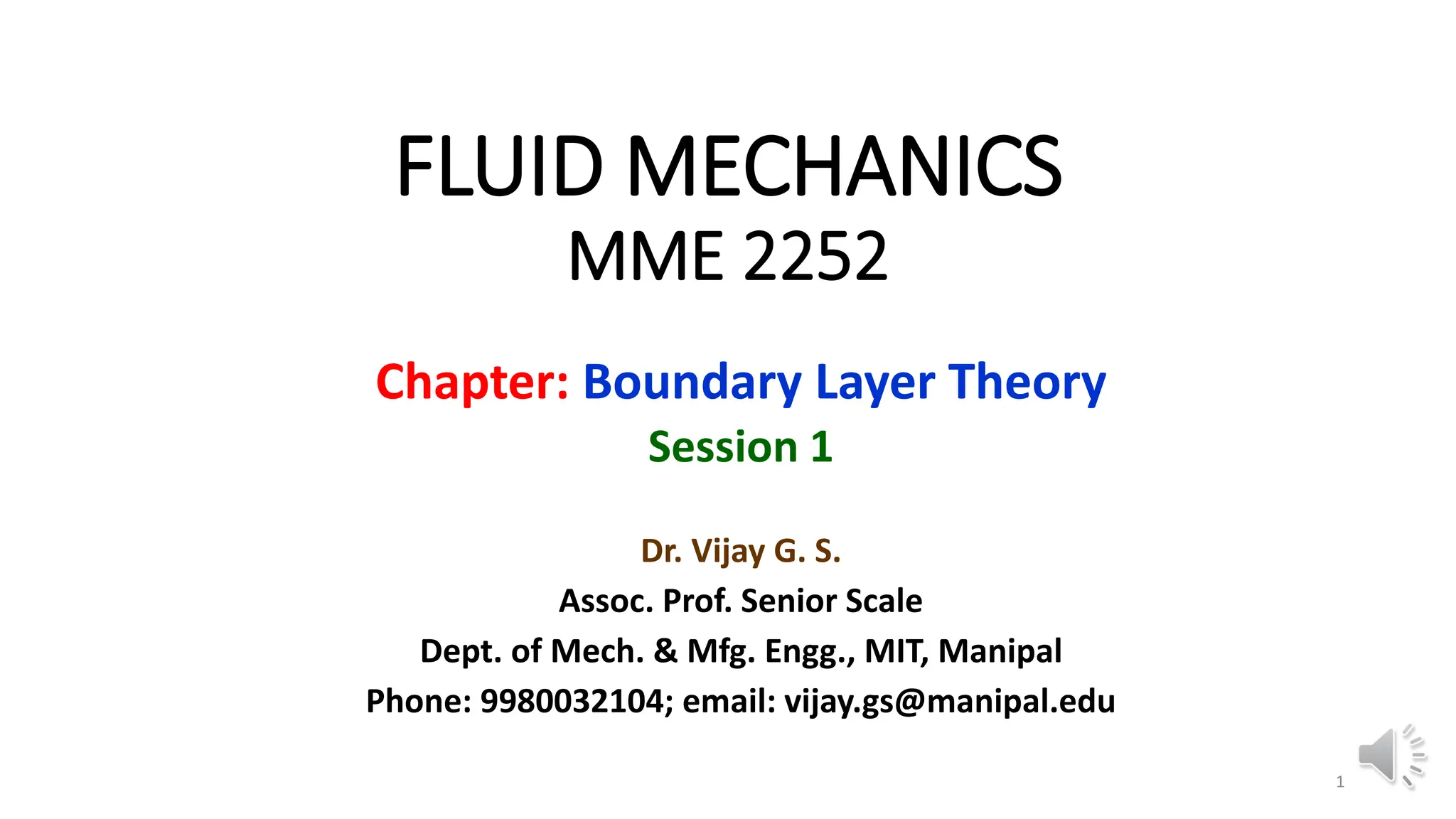
The document provides information about boundary layer theory from a fluid mechanics course. It contains definitions and concepts related to boundary layers, including:
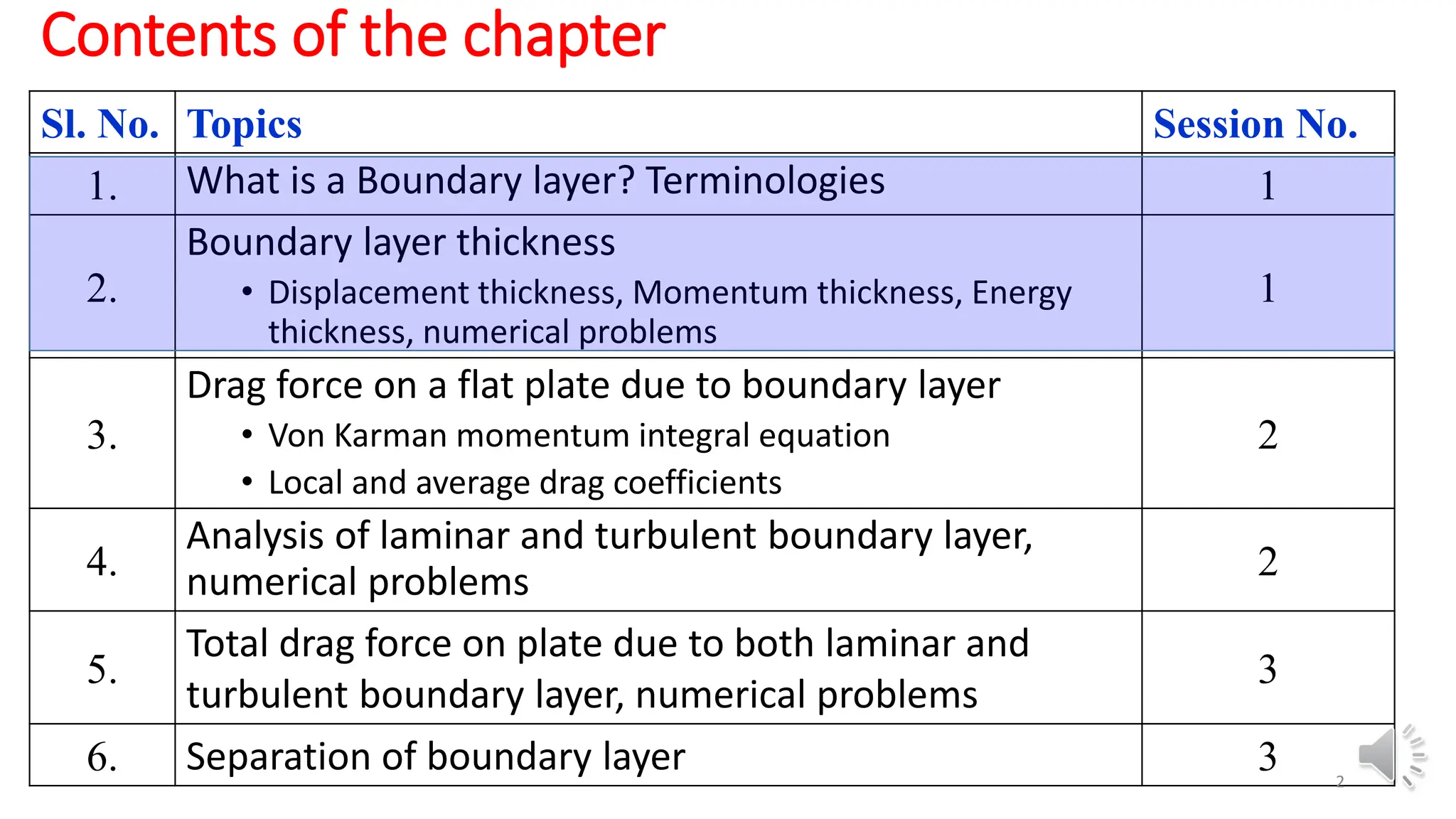
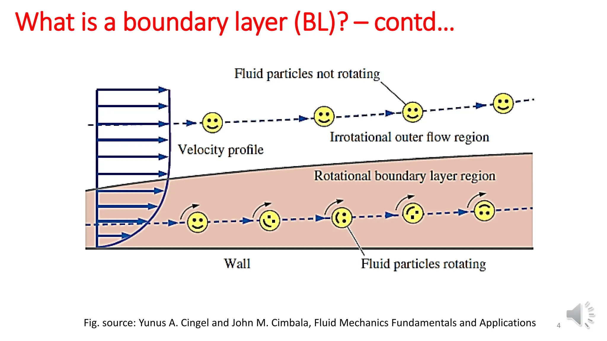
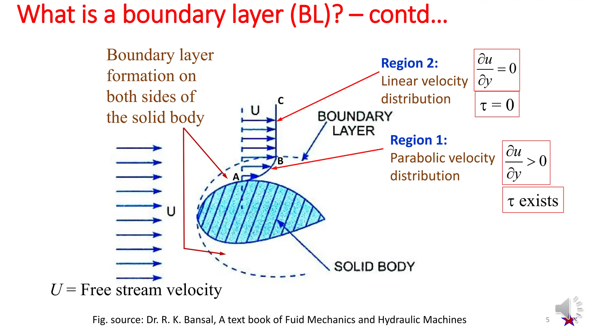
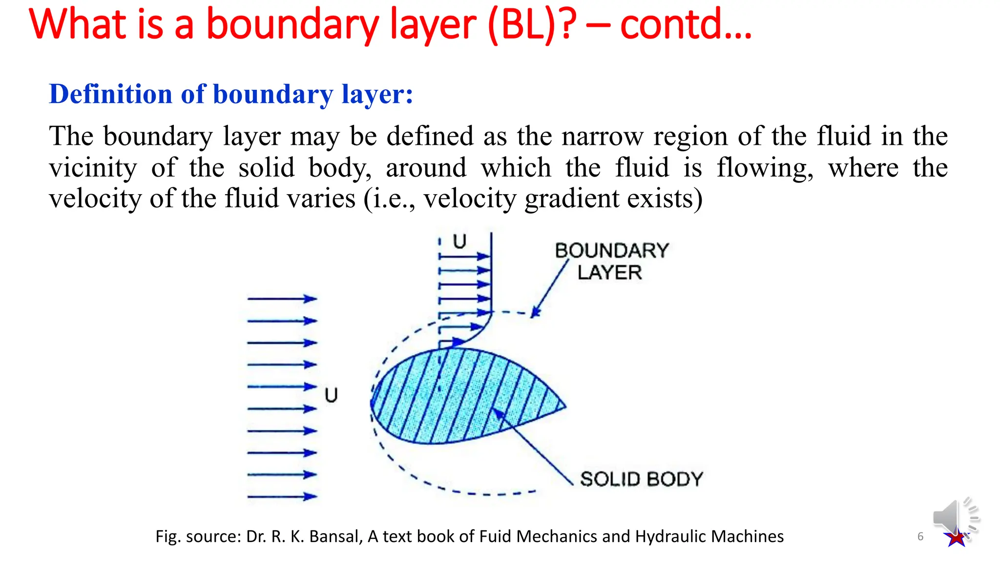
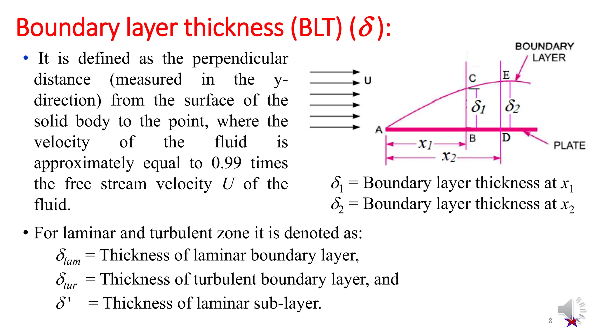
- What constitutes a boundary layer and the velocity profiles within and outside of it.
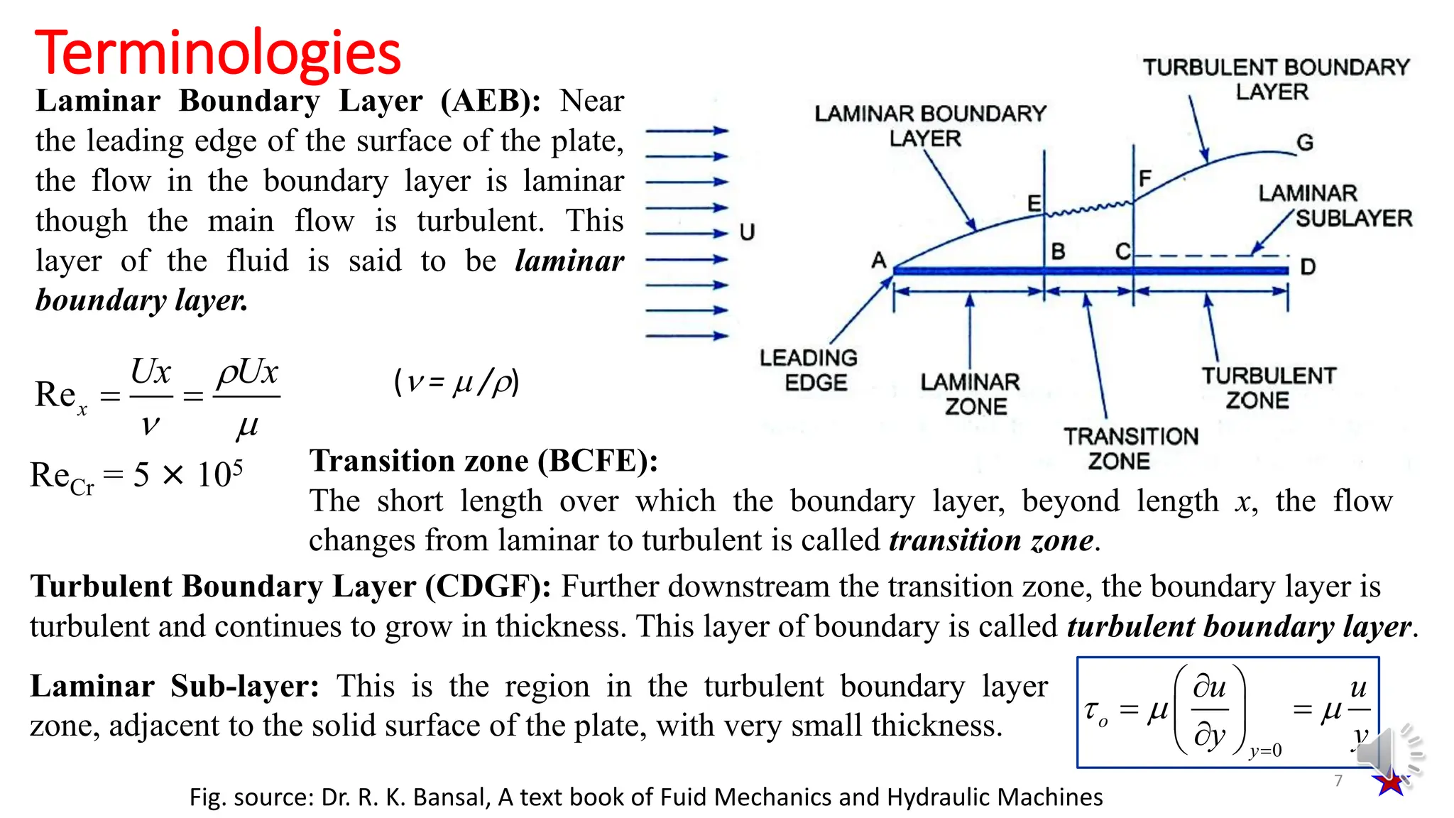
- Key terminologies like laminar boundary layer, transition zone, turbulent boundary layer, and laminar sub-layer.
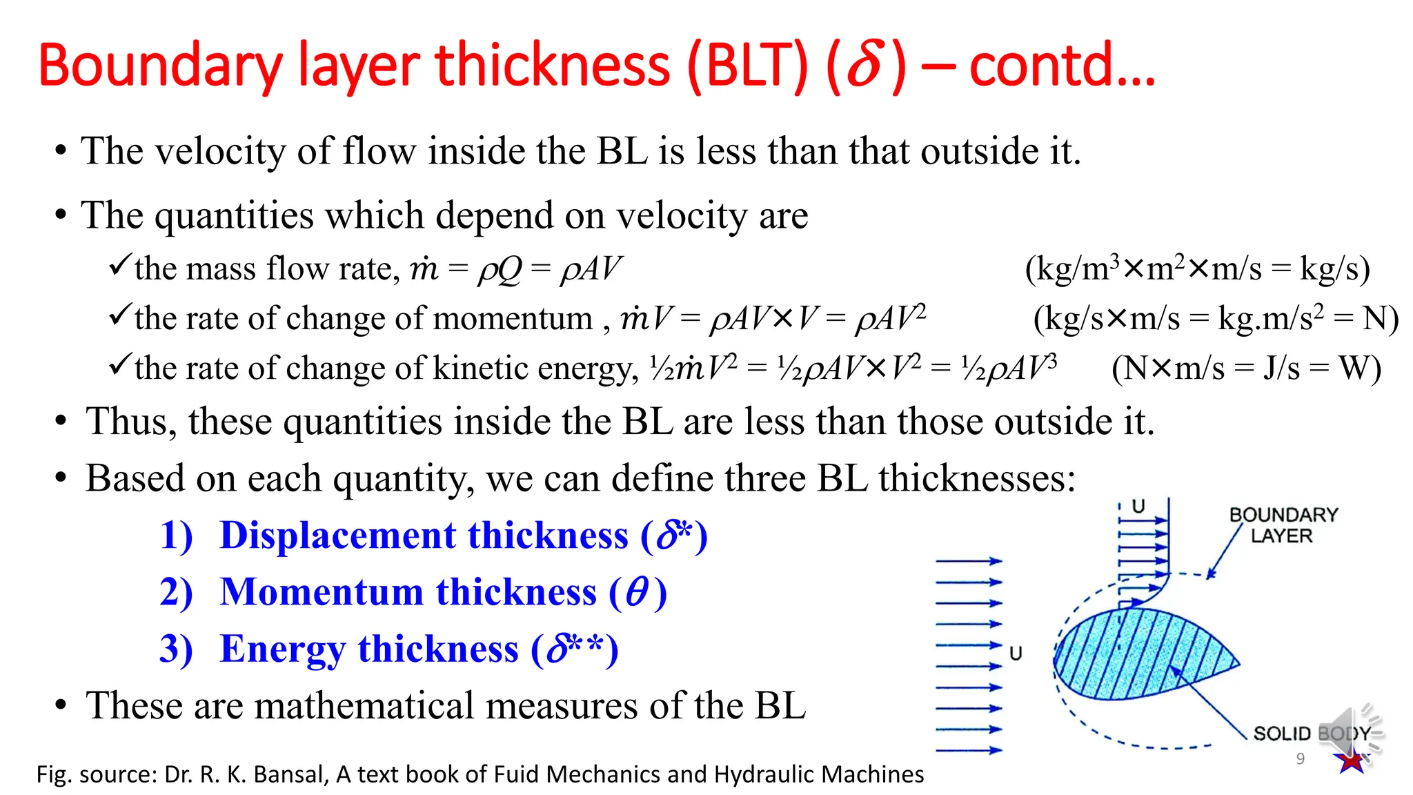
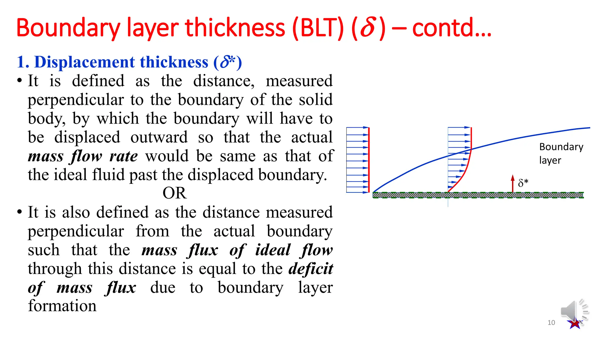
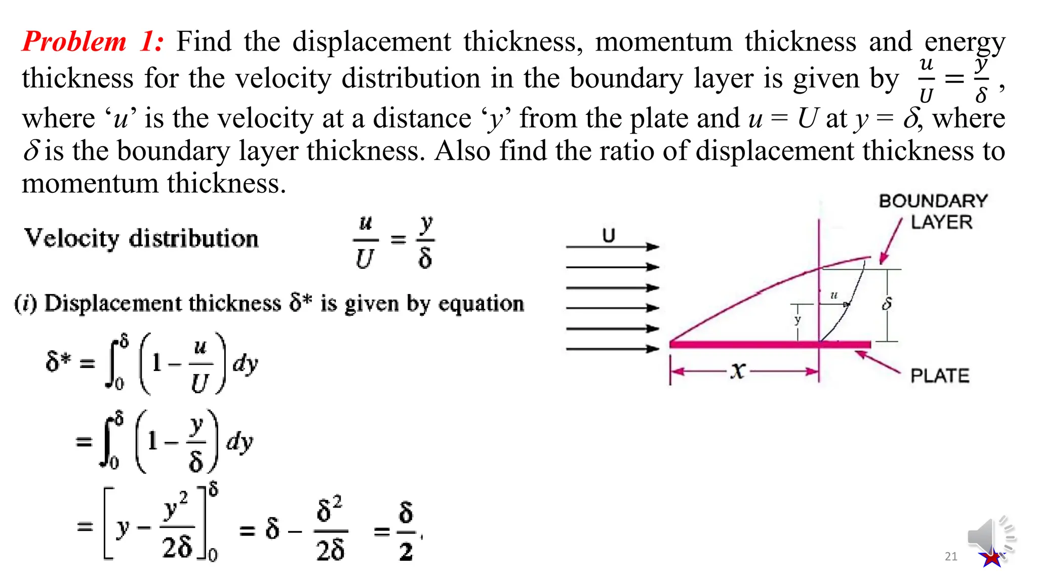
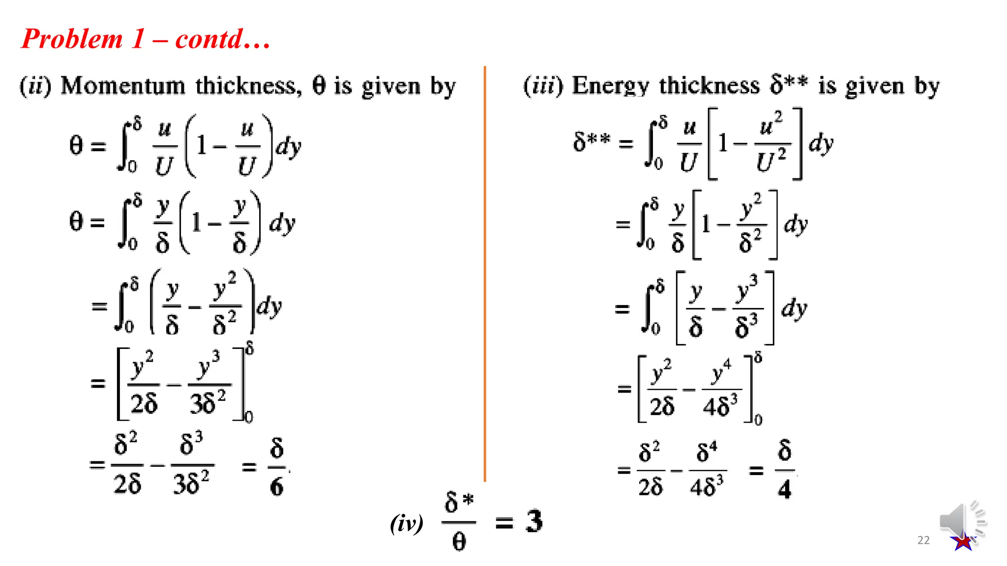
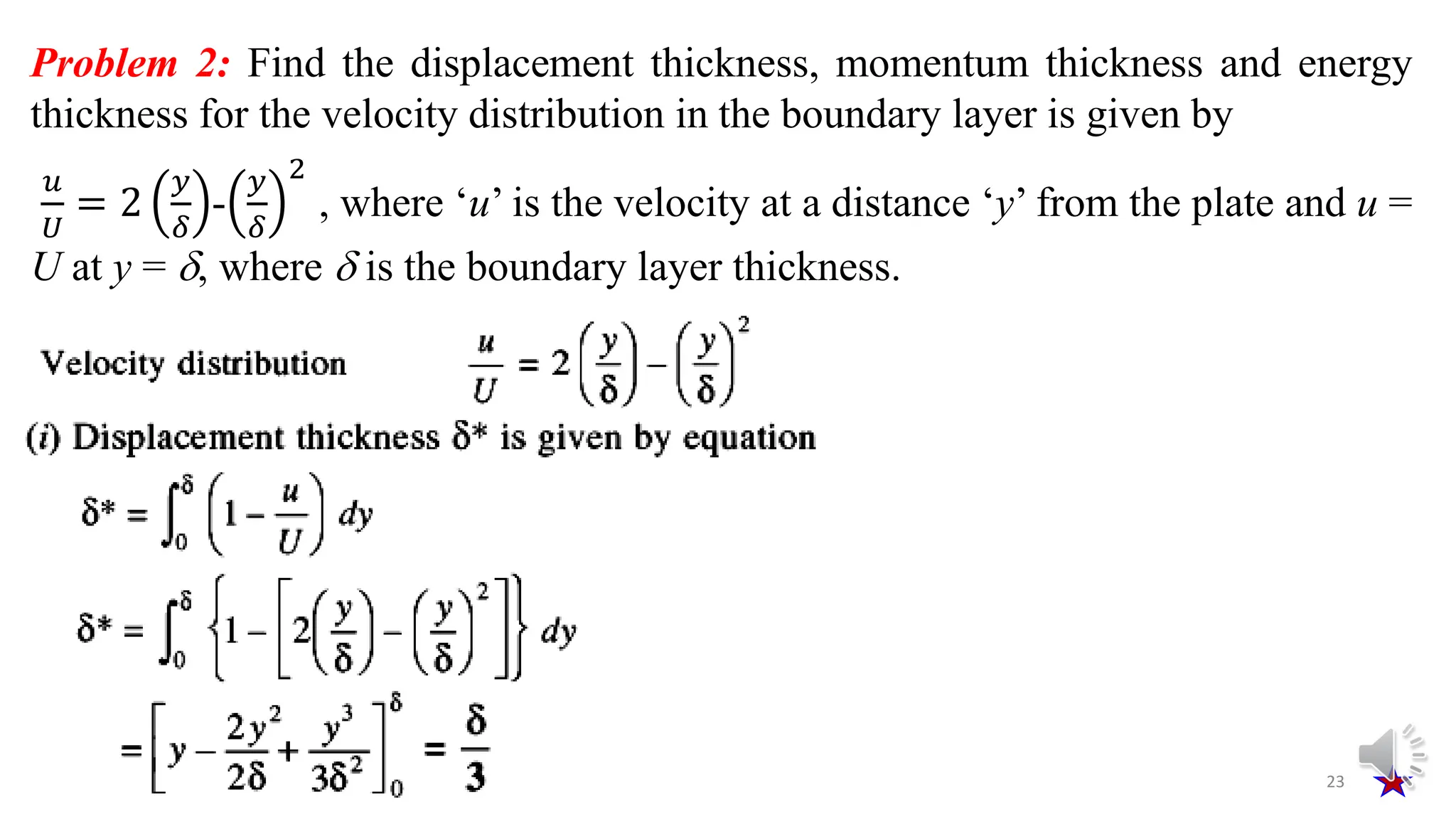
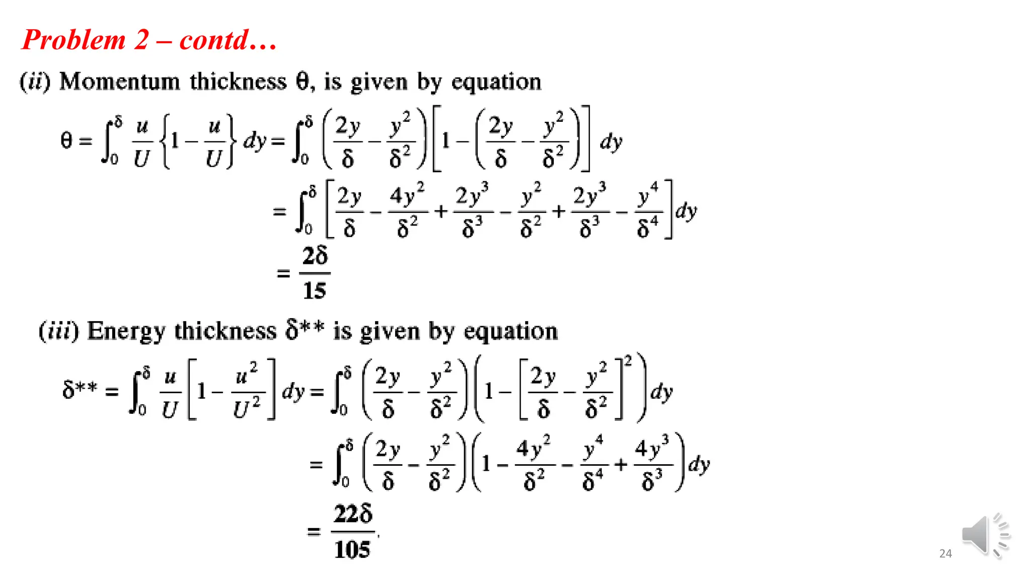
- Definitions and equations for calculating displacement thickness, momentum thickness, and energy thickness, which are measures of the boundary layer.
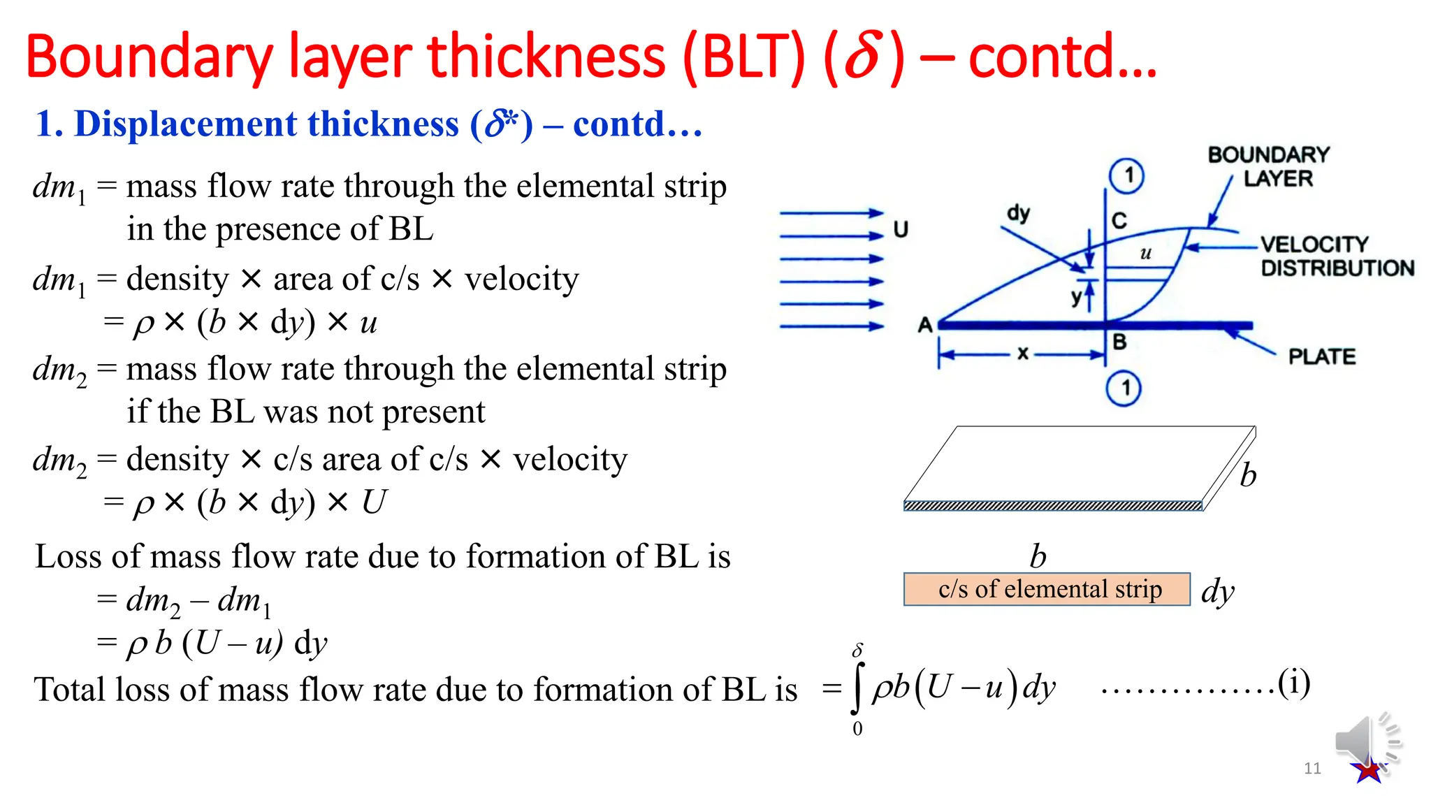
- Explanations and derivations of the equations for displacement thickness, momentum thickness, and energy thickness in terms of the velocity profile within the boundary layer.
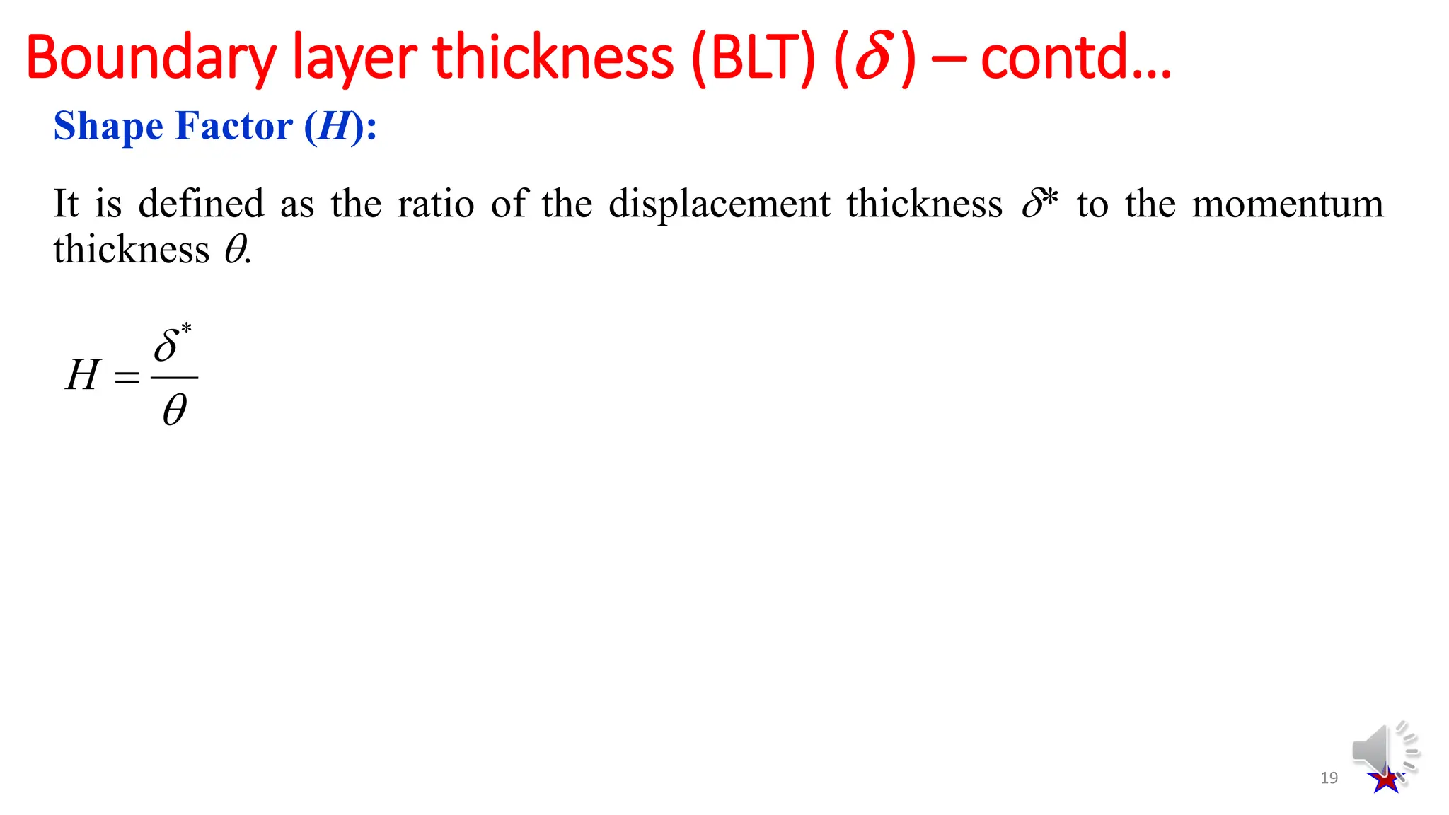
- Introduction of the shape factor H, defined as the ratio of displacement
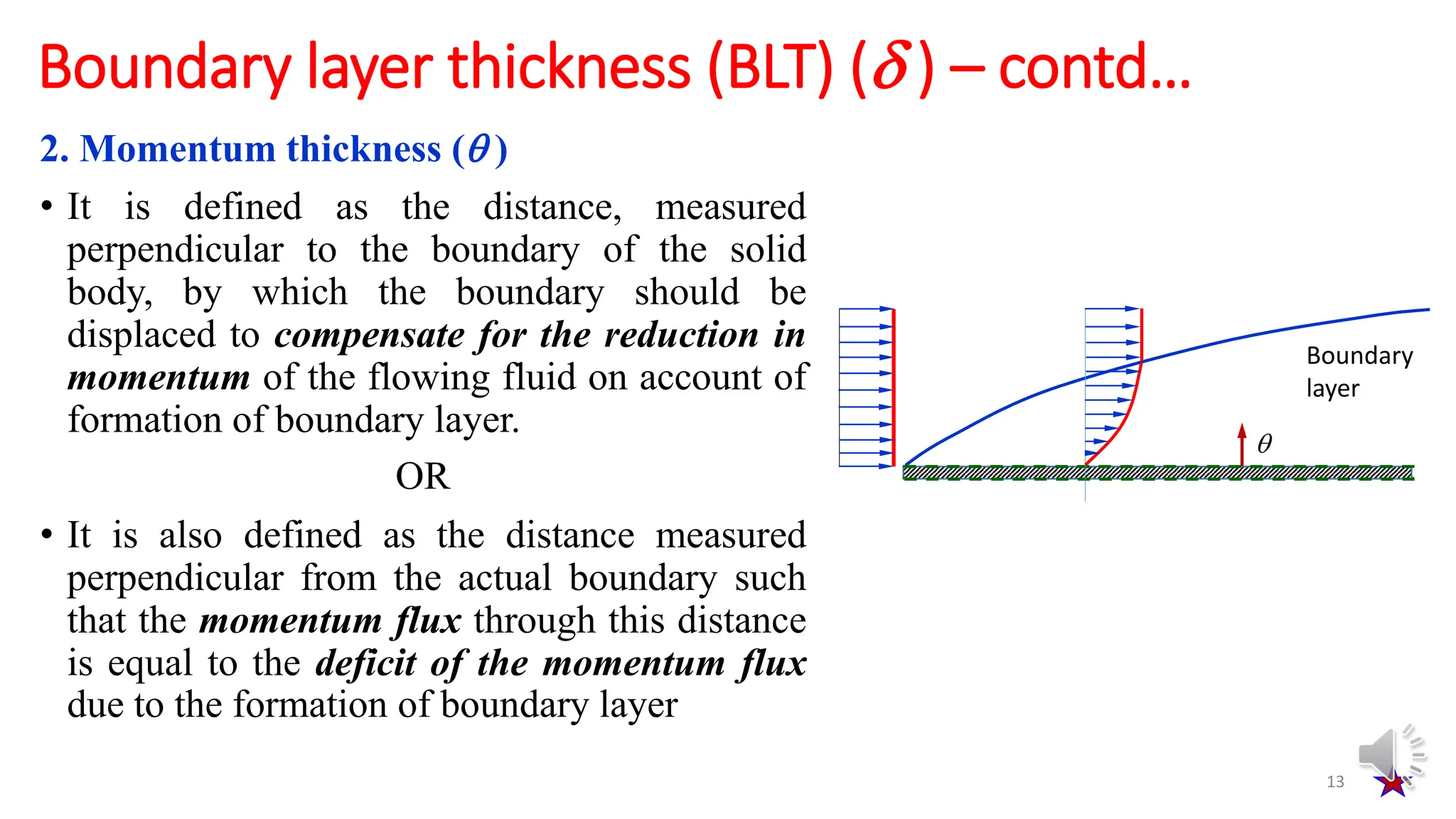
![2. Momentum thickness ( ) – contd…
14
Boundary layer thickness (BLT) ( ) – contd…
dp1 = momentum flux through the elemental
strip in the presence of BL
dp1 = mass flow rate × velocity
= [ × (b × dy) × u] × u
dp2 = momentum flux through the elemental
strip if the BL was not present
dp2 = mass flow rate × velocity
= [ × (b × dy) × u] × U
Loss of momentum flux due to formation of BL is
= dp2 – dp1
= b uU dy - b u2 dy = b (uU – u2) dy
Total loss of momentum flux due to formation of BL is
2
0
b uU u dy
……….(iii)
b
b
dy
c/s of elemental strip
Fig. source: Dr. R. K. Bansal, A text book of Fuid Mechanics and Hydraulic Machines](https://image.slidesharecdn.com/011pptboundarylayerflow-240314062840-d3d66625/75/011-PPT-Boundary-Layer-Flow-pdf-14-2048.jpg)
![15
Boundary layer thickness (BLT) ( ) – contd…
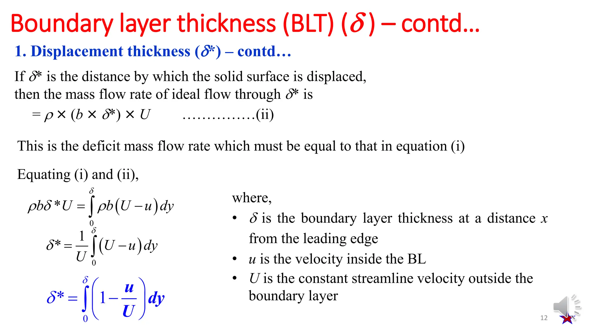
If is the distance by which the solid surface is displaced,
then the momentum flux through is
= mass flow rate × velocity
= [ × (b × ) × U ] × U = b U2 ……………(iv)
This is the deficit of the momentum flux which must be equal to that in equation (iii)
Equating (iii) and (iv),
2 2
0
b U b uU u dy
2
2
2
0 0
1 u u
uU u dy dy
U U U
0
1
u u
dy
U U
where,
• is the boundary layer thickness at a
distance x from the leading edge
• u is the velocity inside the BL
• U is the constant streamline velocity
outside the boundary layer
2. Momentum thickness ( ) – contd…](https://image.slidesharecdn.com/011pptboundarylayerflow-240314062840-d3d66625/75/011-PPT-Boundary-Layer-Flow-pdf-15-2048.jpg)
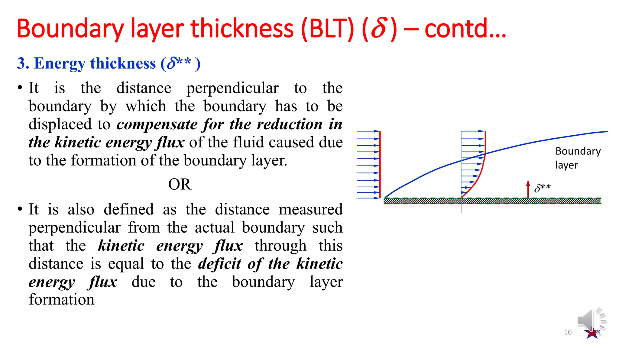
![3. Energy thickness (** ) – contd…
17
Boundary layer thickness (BLT) ( ) – contd…
dKE1 = KE flux through the elemental strip in
the presence of BL
dKE1 = ½ × mass flow rate × velocity2
= ½ × [ × (b × dy) × u ] × u2
dKE2 = KE flux through the elemental strip if the
BL was not present
dKE2 = ½ × mass flow rate × velocity2
= ½ × [ × (b × dy) × u ] × U2
Loss of KE flux due to formation of BL is
= dKE2 – dKE1
= ½ [ b uU2 dy - b u3 dy = ½ b (uU2 – u3) dy
Total loss of KE flux due to formation of BL is
2 3
0
1
2
b uU u dy ……………(v)
b
b
dy
c/s of elemental strip
Fig. source: Dr. R. K. Bansal, A text book of Fuid Mechanics and Hydraulic Machines](https://image.slidesharecdn.com/011pptboundarylayerflow-240314062840-d3d66625/75/011-PPT-Boundary-Layer-Flow-pdf-17-2048.jpg)
![18
Boundary layer thickness (BLT) ( ) – contd…
If ** is the distance by which the solid surface is displaced,
then the KE flux through ** is
= ½ × mass flow rate × velocity2
= ½ × [ × (b × ** ) × U ] × U2 = ½ b ** U3 ……………(vi)
This is the deficit of the KE flux which must be equal to that in equation (v)
Equating (v) and (vi),
3 2 3
0
1 1
**
2 2
b U b uU u dy
3
2 3
3
0 0
1
**
u u
uU u dy dy
U U U
2
0
** 1
u u
dy
U U
where,
• is the boundary layer thickness at a
distance x from the leading edge
• u is the velocity inside the BL
• U is the constant streamline velocity
outside the boundary layer
3. Energy thickness (** ) – contd…](https://image.slidesharecdn.com/011pptboundarylayerflow-240314062840-d3d66625/75/011-PPT-Boundary-Layer-Flow-pdf-18-2048.jpg)
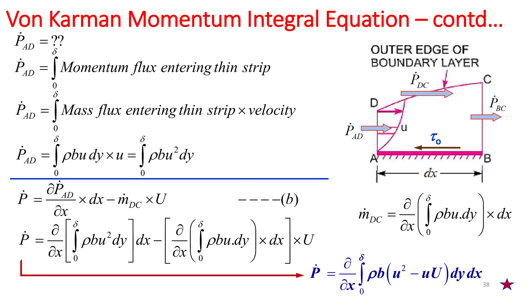
![37
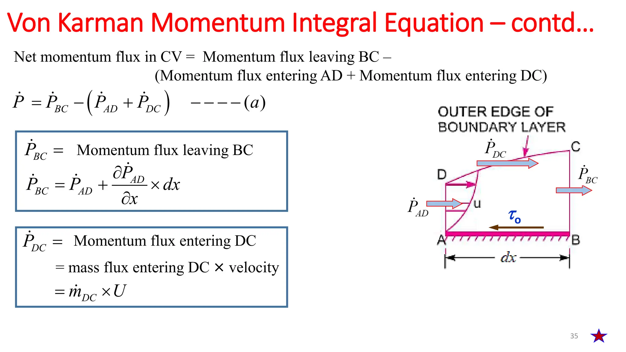
Von Karman Momentum Integral Equation – contd…
??
DC
m
0
.
AD AD
DC BC AD AD AD
m m
m m m m dx m dx bu dy dx
x x x
AD
BC AD
m
m m dx
x
Let d ሶ
𝑚 = Mass flux through elemental strip of thickness dy
d ሶ
𝑚 = × dQ = × (area of elemental strip × velocity)
d ሶ
𝑚 = × [(b × dy) × u)]
0
. ( )
AD
m bu dy c
Find AD
m
Consider thin strip of thickness dy at distance y, here velocity = u
Find BC
m
BC AD DC
m m m
DC BC AD
m m m
](https://image.slidesharecdn.com/011pptboundarylayerflow-240314062840-d3d66625/75/011-PPT-Boundary-Layer-Flow-pdf-37-2048.jpg)