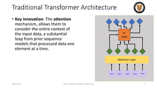
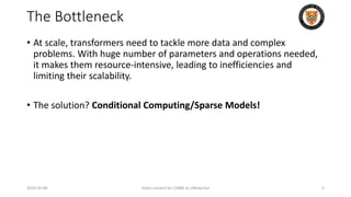
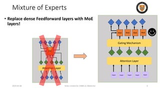
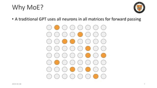
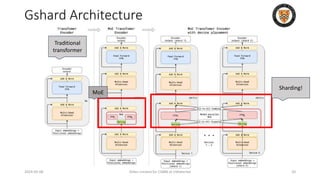
The lecture discusses recent advancements in compressing and sparsifying large language models (LLMs), focusing on techniques such as mixtures of experts (MoE) and the GShard architecture which enhance efficiency and scalability. Key insights include the use of conditional computation to improve processing efficiency by selectively utilizing model components, alongside exploration of models like COLT5 that optimize for handling long inputs. The aim is to achieve similar performance to traditional models while significantly reducing computational costs and resource consumption.
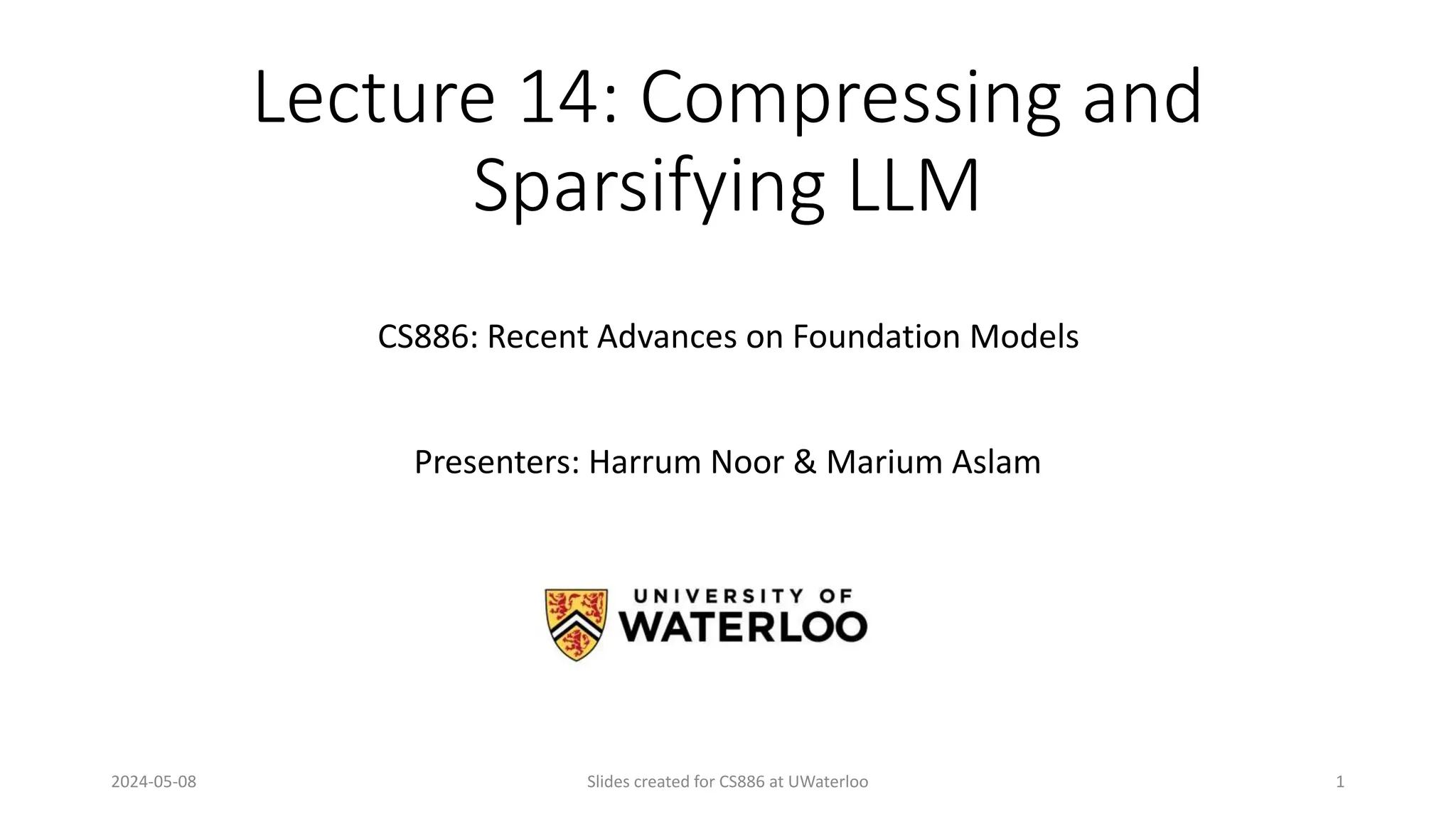
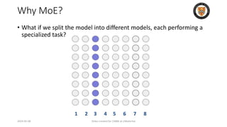
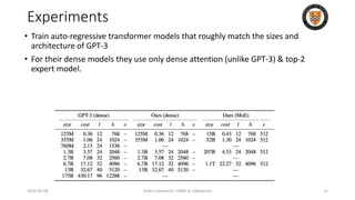
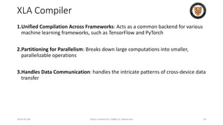
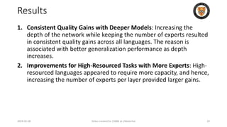
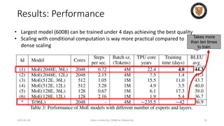
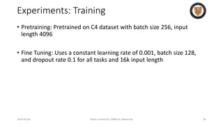
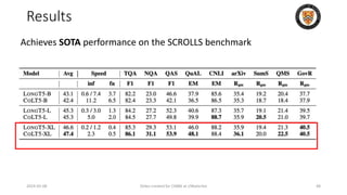
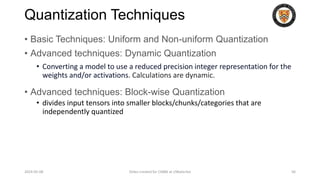
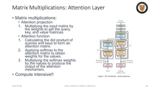
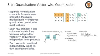
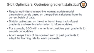
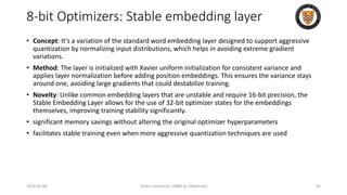
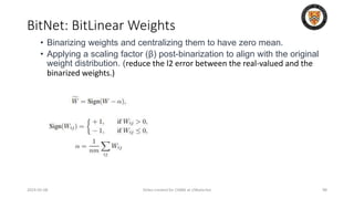
![8-bit Optimizers: Block-wise Quantization
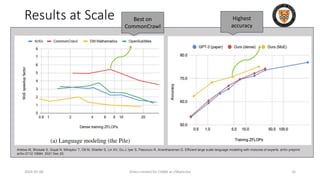
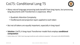
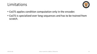
• isolates outliers and distributes the error more equally over all bits
• Breaks down a tensor into smaller blocks, normalizing each block
independently for efficient computation and processed in parallel
• Dynamic Range Adjustment: Each block's values are normalized within the
range [-1, 1], using the maximum value within that block as a reference.
• Tqbi: The quantized value of tensor T for block b at index i.
• Qmapj: A function mapping the j-th element to its quantized form.
• Nb: The normalization constant for block b, which is the maximum
absolute value within that block.
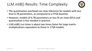
2024-05-08 Slides created for CS886 at UWaterloo 78](https://image.slidesharecdn.com/l14-240508092129-be2669b5/85/Compressing-and-Sparsifying-LLM-in-GenAI-Applications-78-320.jpg)

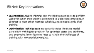
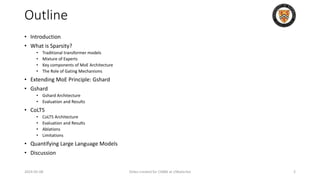
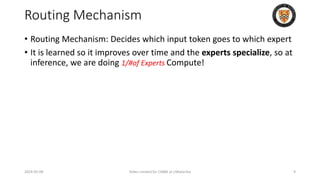
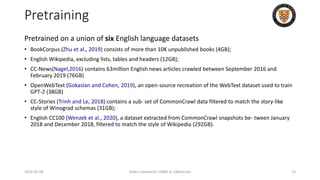
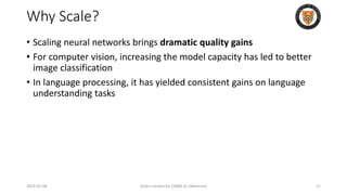
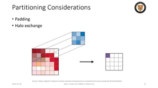
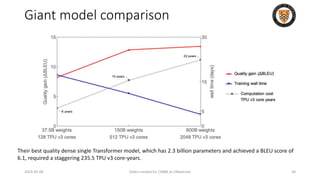
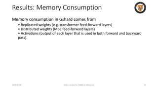
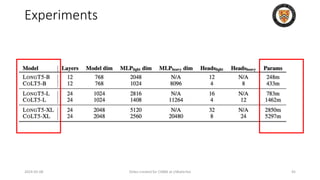
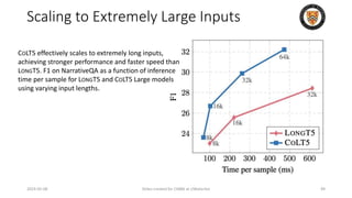
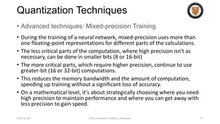
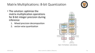
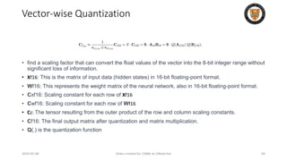
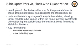
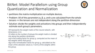
![BitNet: BitLinear Activations
2024-05-08 Slides created for CS886 at UWaterloo 99
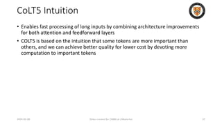
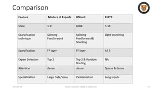
• Activation functions are quantized to b-bit precision via absmax
while ensuring the output's variance is maintained for stability.
• Scaled to Range [-Qb, Qb]
• Multiply by 2b-1 and divide by maximum
• Qb = 2b-1
• Activations before non-linear functions are scaled onto the range
[0, Q8] by subtracting the minimum of the inputs so that all values are
non-negative.](https://image.slidesharecdn.com/l14-240508092129-be2669b5/85/Compressing-and-Sparsifying-LLM-in-GenAI-Applications-99-320.jpg)
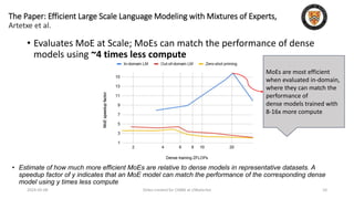
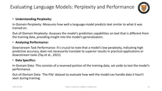
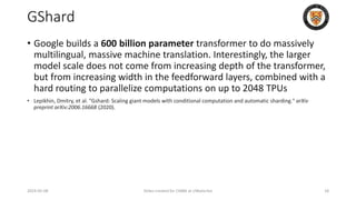
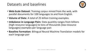
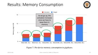
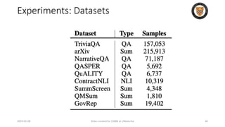
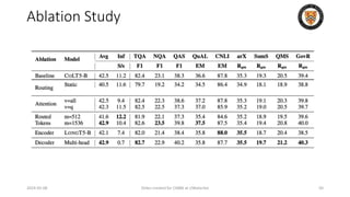
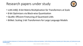
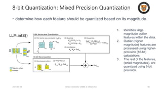
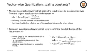
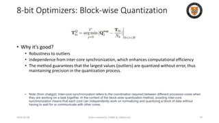
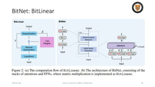
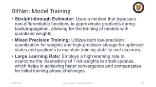
![BitNet: BitLinear
2024-05-08 Slides created for CS886 at UWaterloo 100
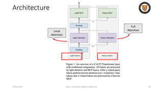
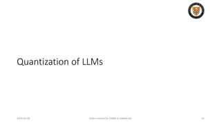
• the matrix multiplication can be written as: 𝑦 = 𝑤𝑥
• assume that the elements in W and x are mutually independent and
share the same distribution, Var(y) is estimated to be:
• After layer norm: Var(y) ≈ E[LN(xe) 2 ] = 1
• BitLinear:](https://image.slidesharecdn.com/l14-240508092129-be2669b5/85/Compressing-and-Sparsifying-LLM-in-GenAI-Applications-100-320.jpg)


![[Harvard CS264] 03 - Introduction to GPU Computing, CUDA Basics](https://cdn.slidesharecdn.com/ss_thumbnails/cs264201103-cudabasicsshare-110209024624-phpapp02-thumbnail.jpg?width=640&height=640&fit=bounds)


