Download as PDF, PPTX


The document provides an overview of multiphase flows, detailing different models like Euler-Lagrange and Euler-Euler, as well as key parameters such as volume fractions, particulate loading, and phase velocities. It explains fundamental definitions and classifications, including dilute and dense flows, and the impact of Stokes number on particle behavior. Additionally, it discusses the application contexts for various multiphase models, guiding the choice of model based on flow characteristics and particle interactions.
Introduction to multiphase flows and presenter details.
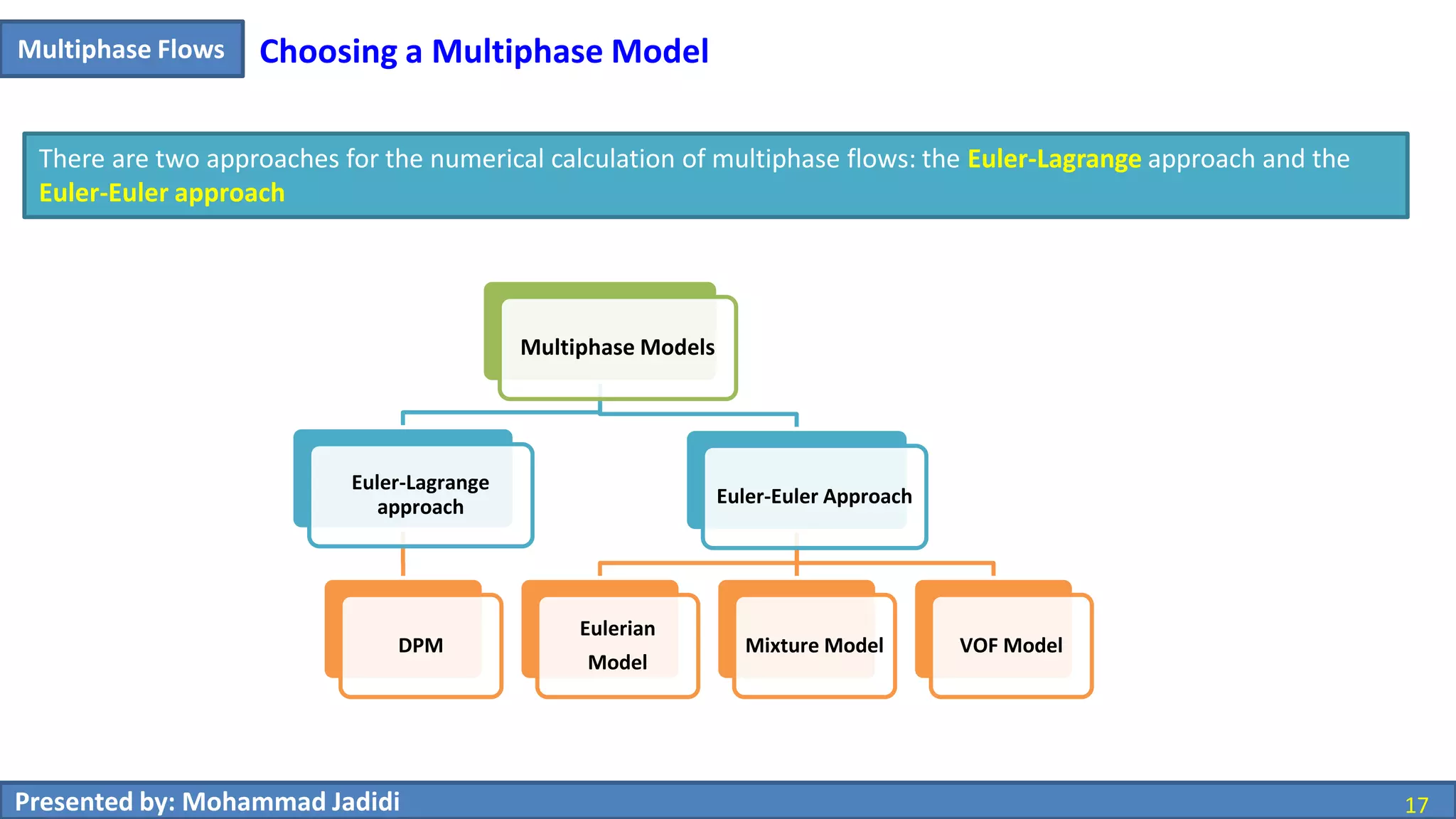
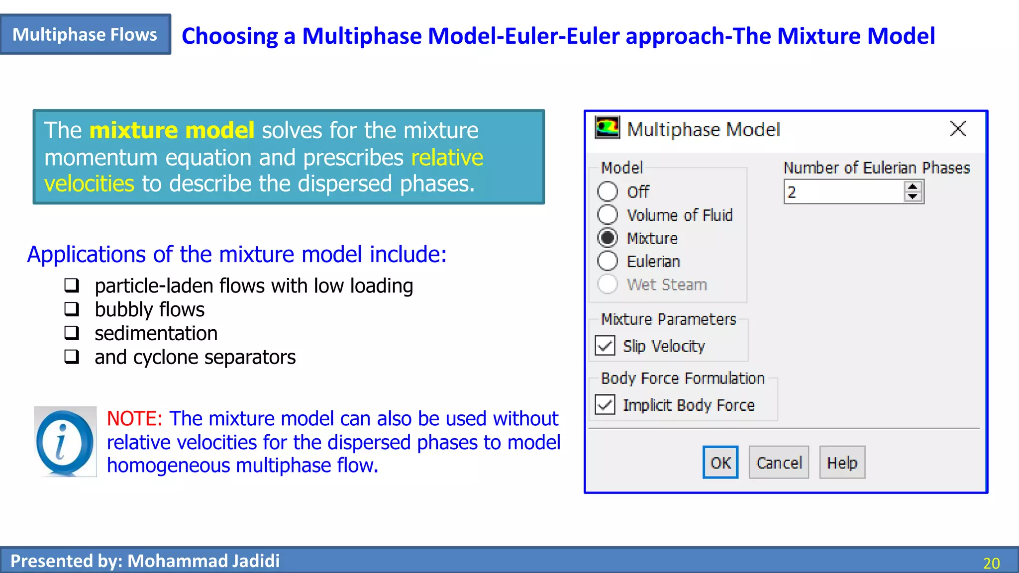
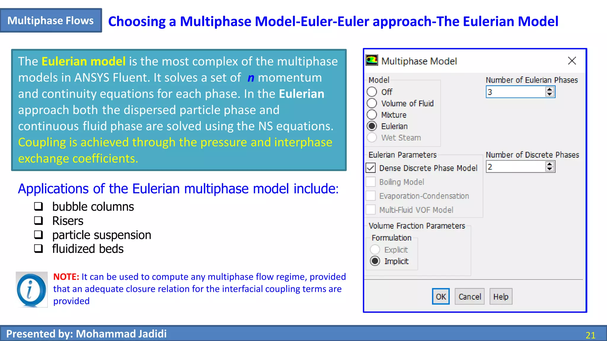
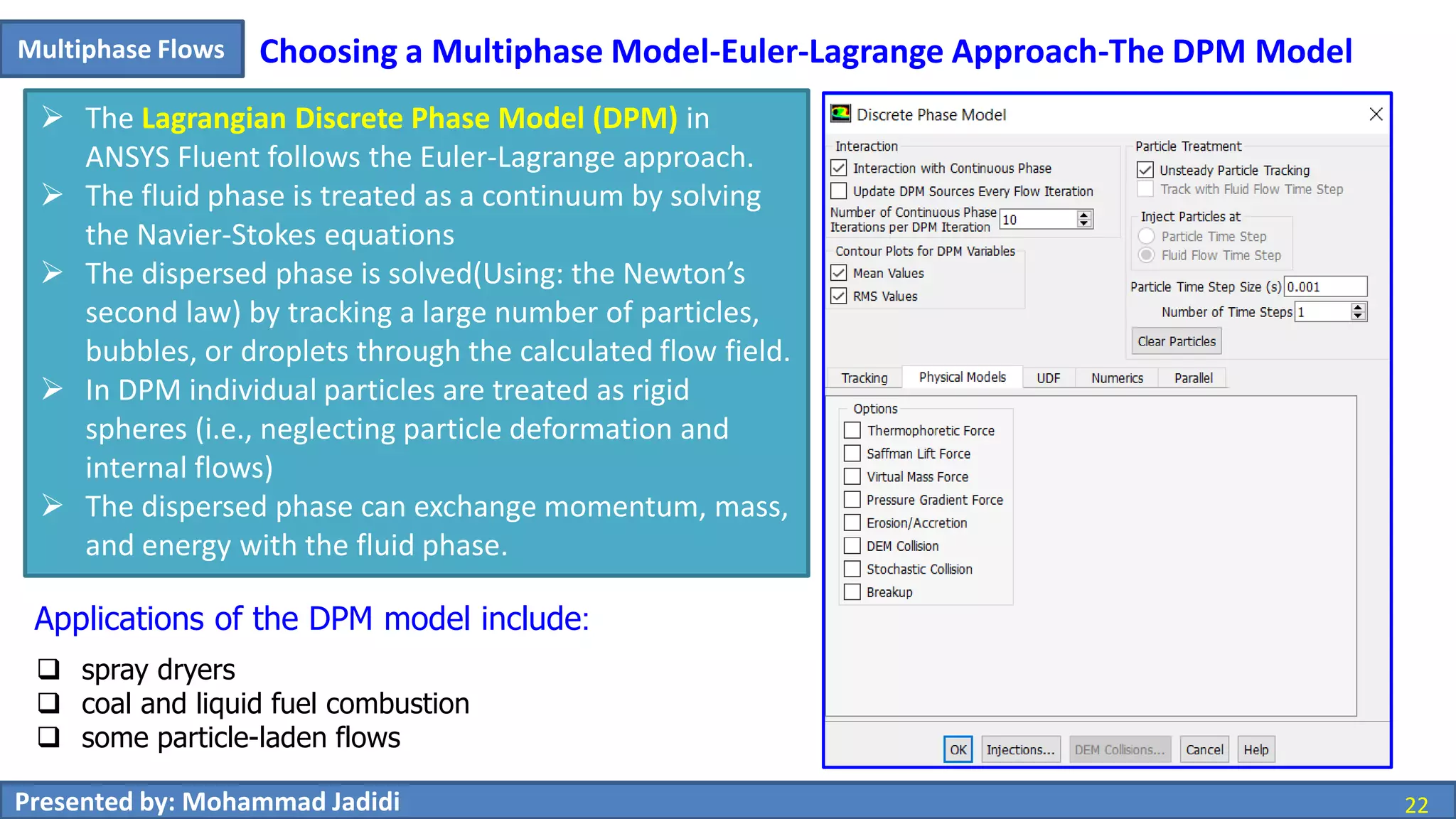
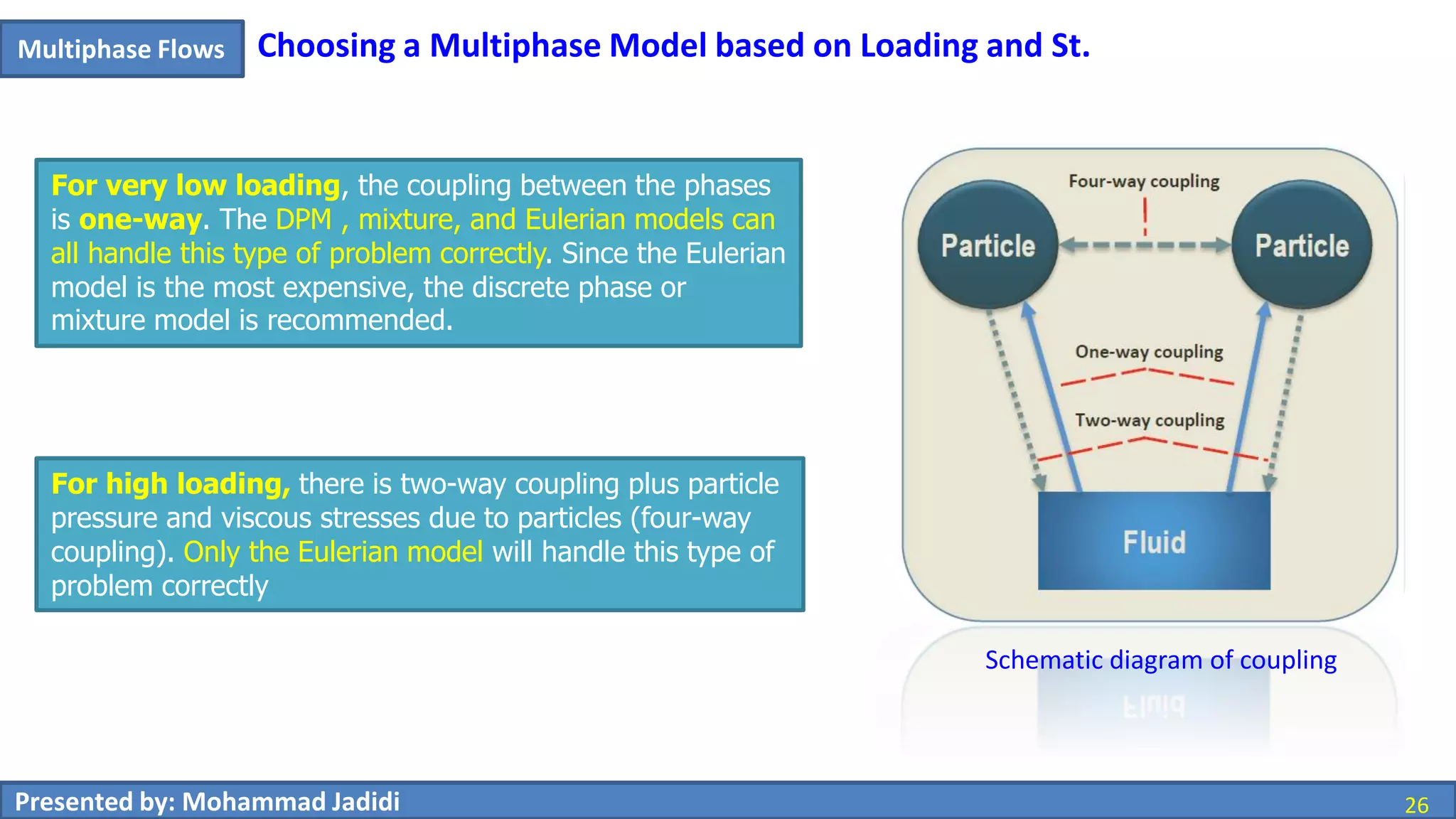
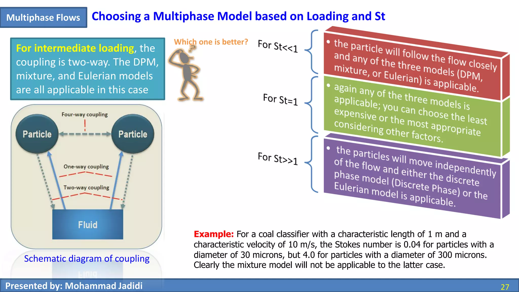
Guidance on selecting multiphase models based on flow parameters like loading, velocities, and phase coupling.
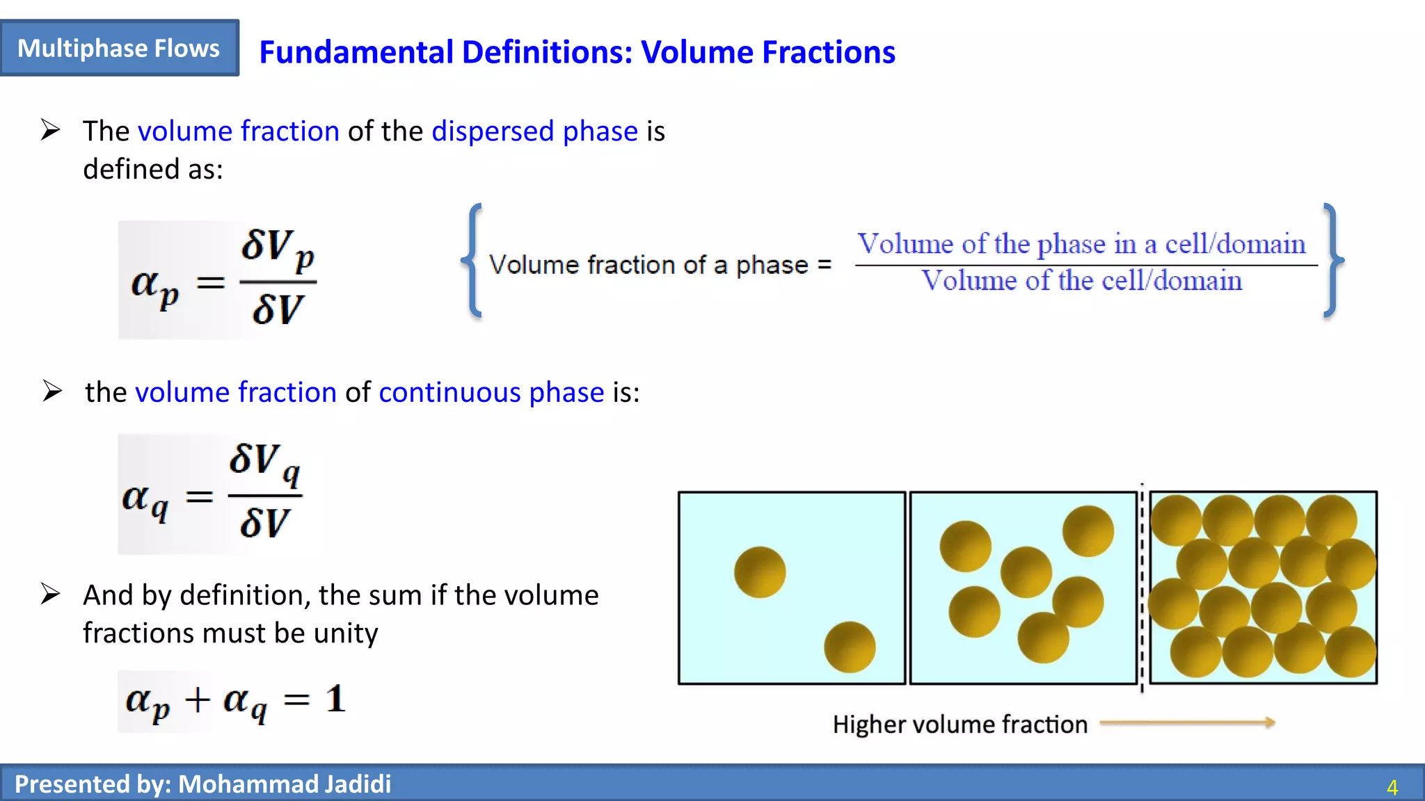
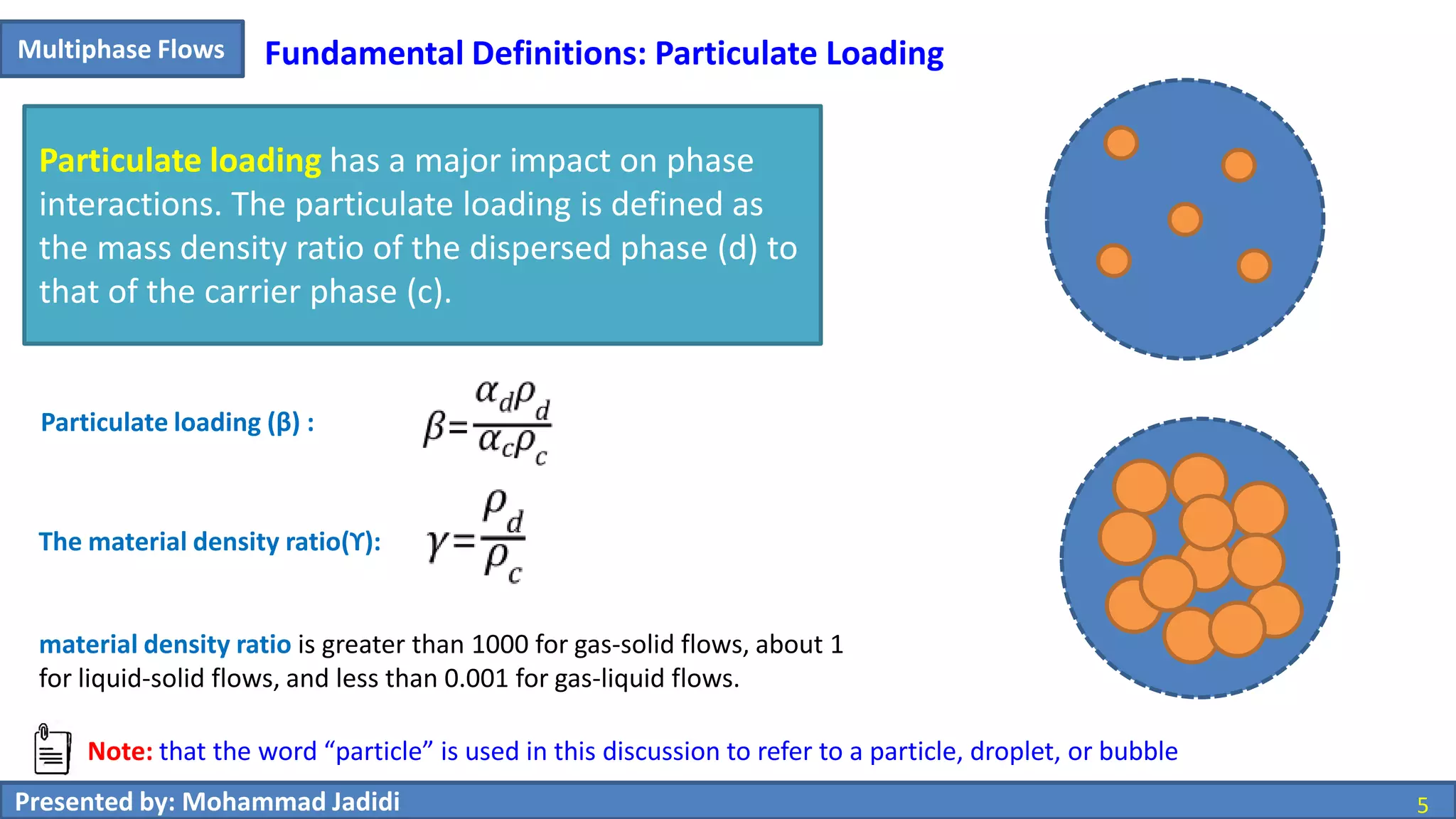
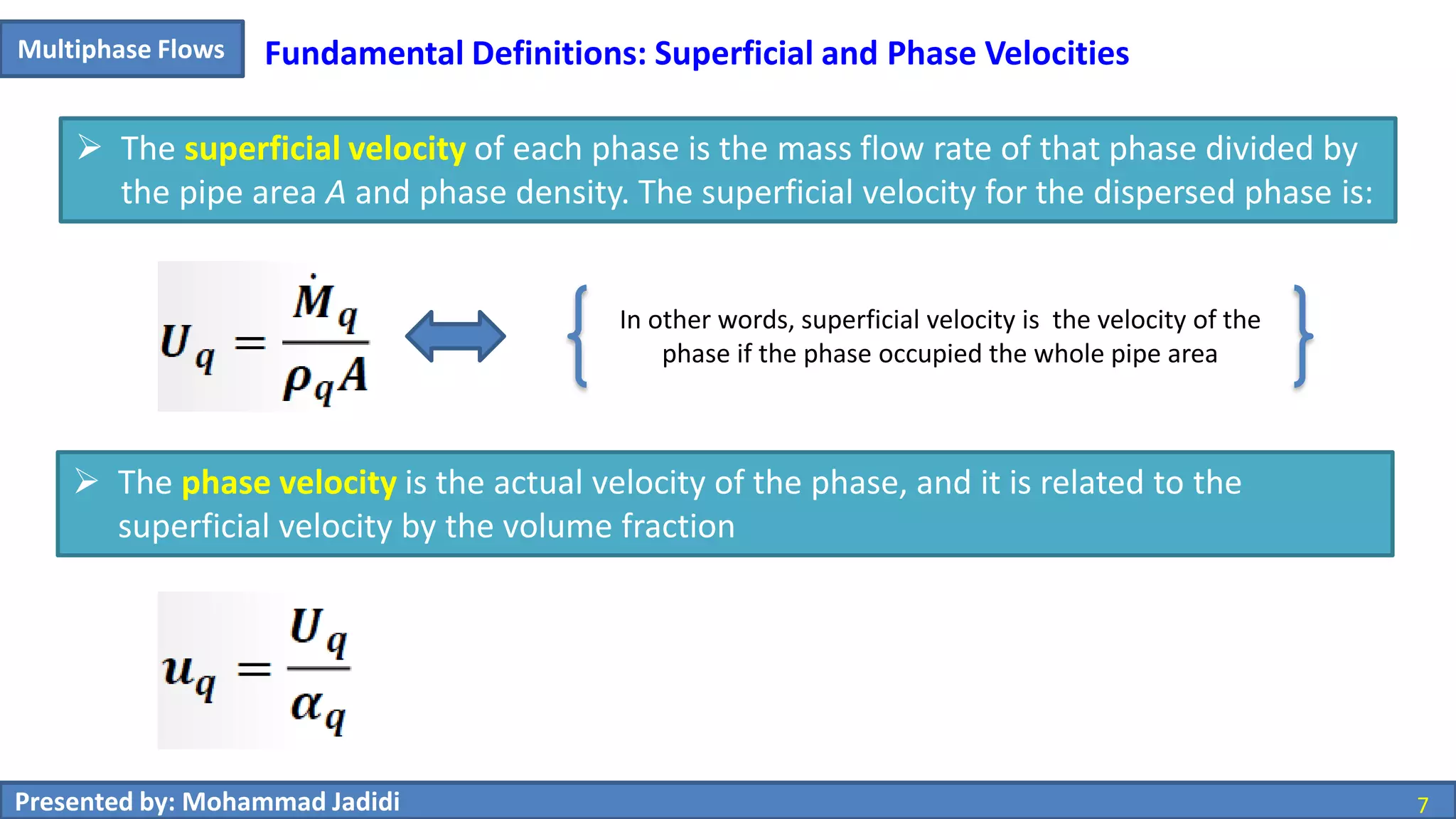
Definitions of primary/secondary phases, volume fractions, particulate loading, and their significance in multiphase flows.
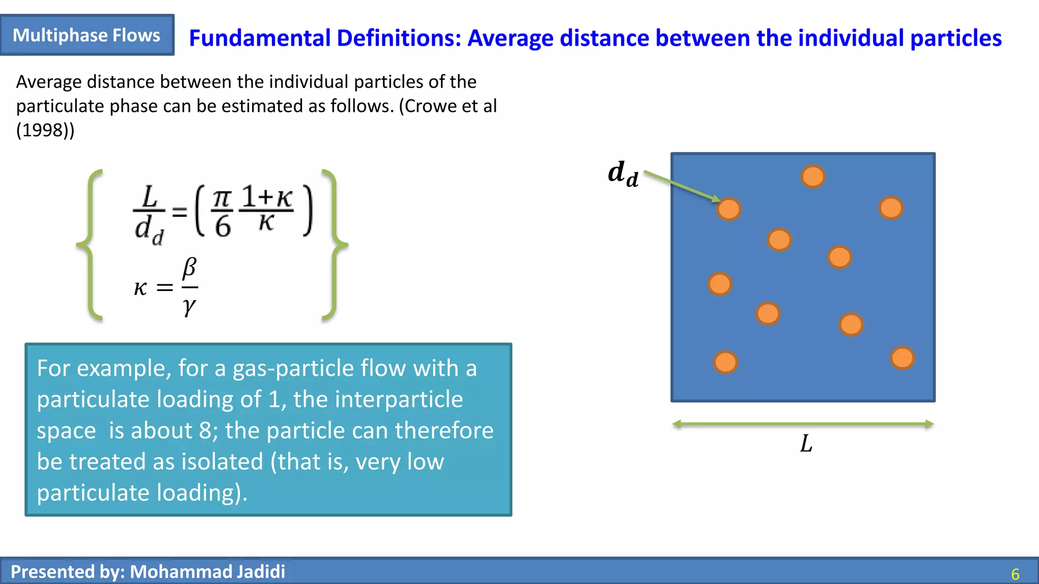
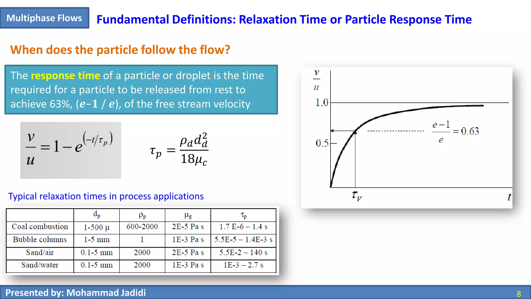
Concepts of mean distance between particles, relaxation time, and their impact on flow dynamics.
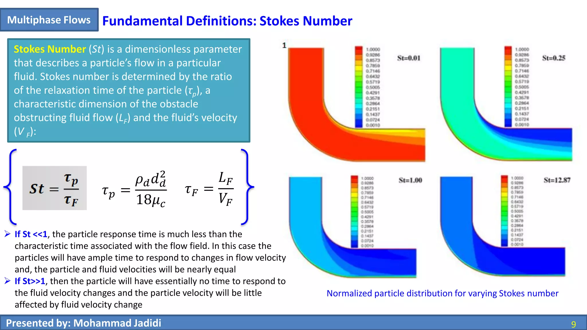
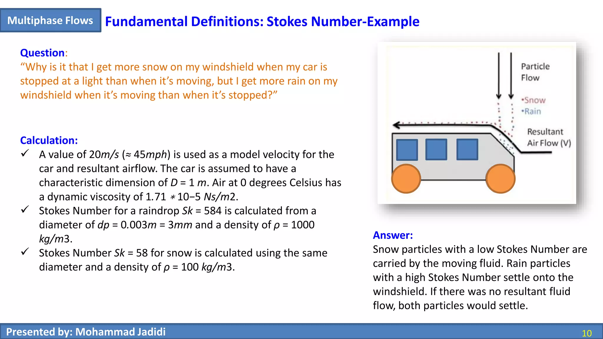
Definition and significance of Stokes number in flow dynamics, with an illustrative example comparing snow and rain.
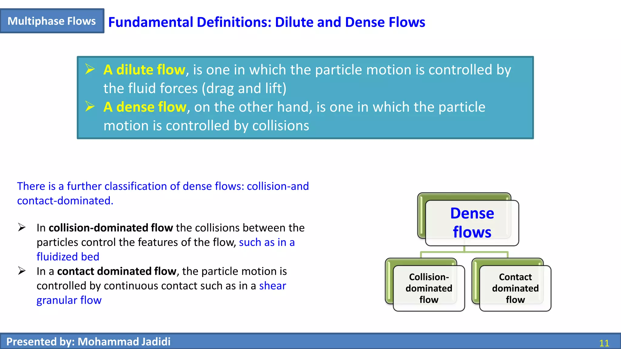
Distinction between dilute and dense flows based on control factors like particle motion and collision.
Detailed overview of different coupling types (one-way, two-way, four-way) and their relevance in multiphase modeling.
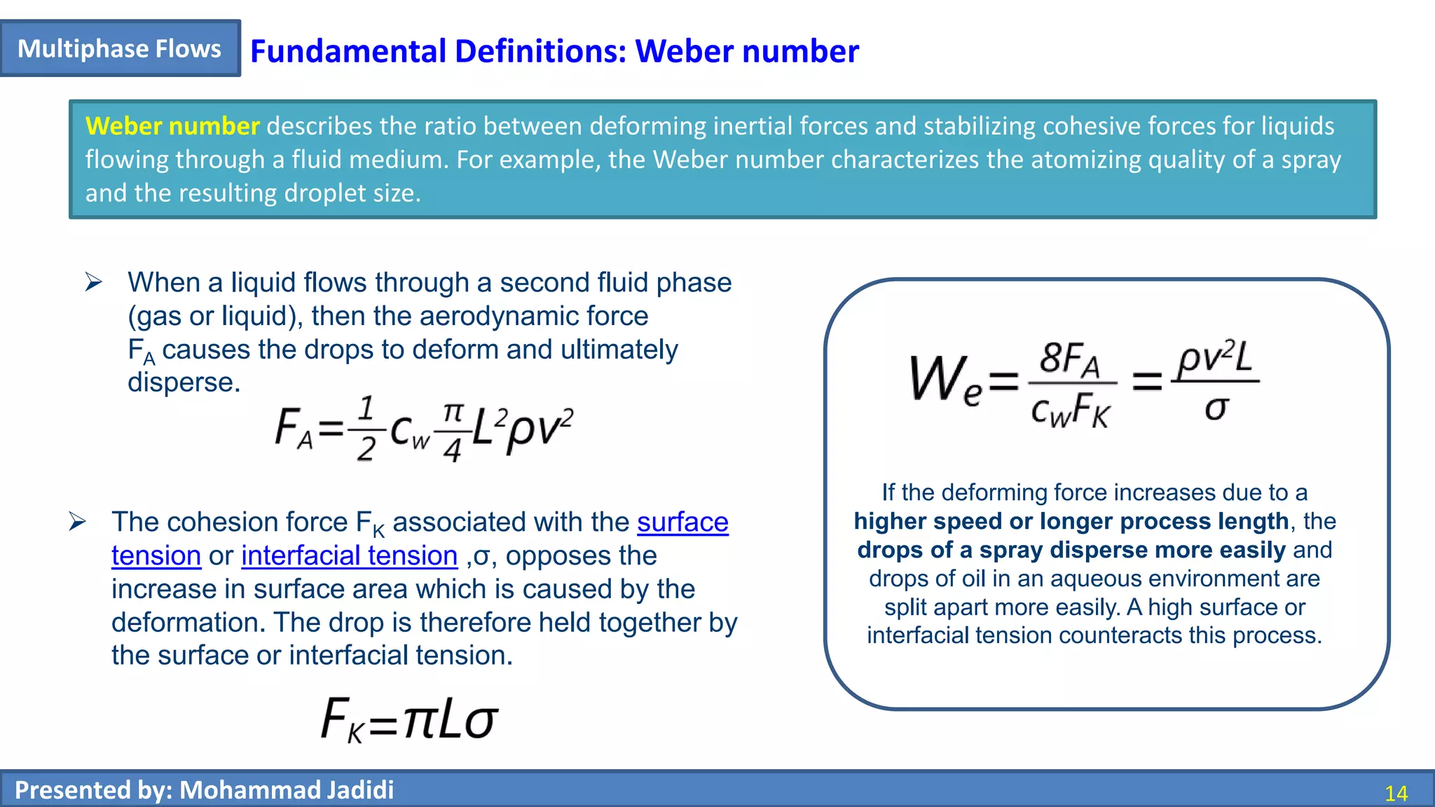
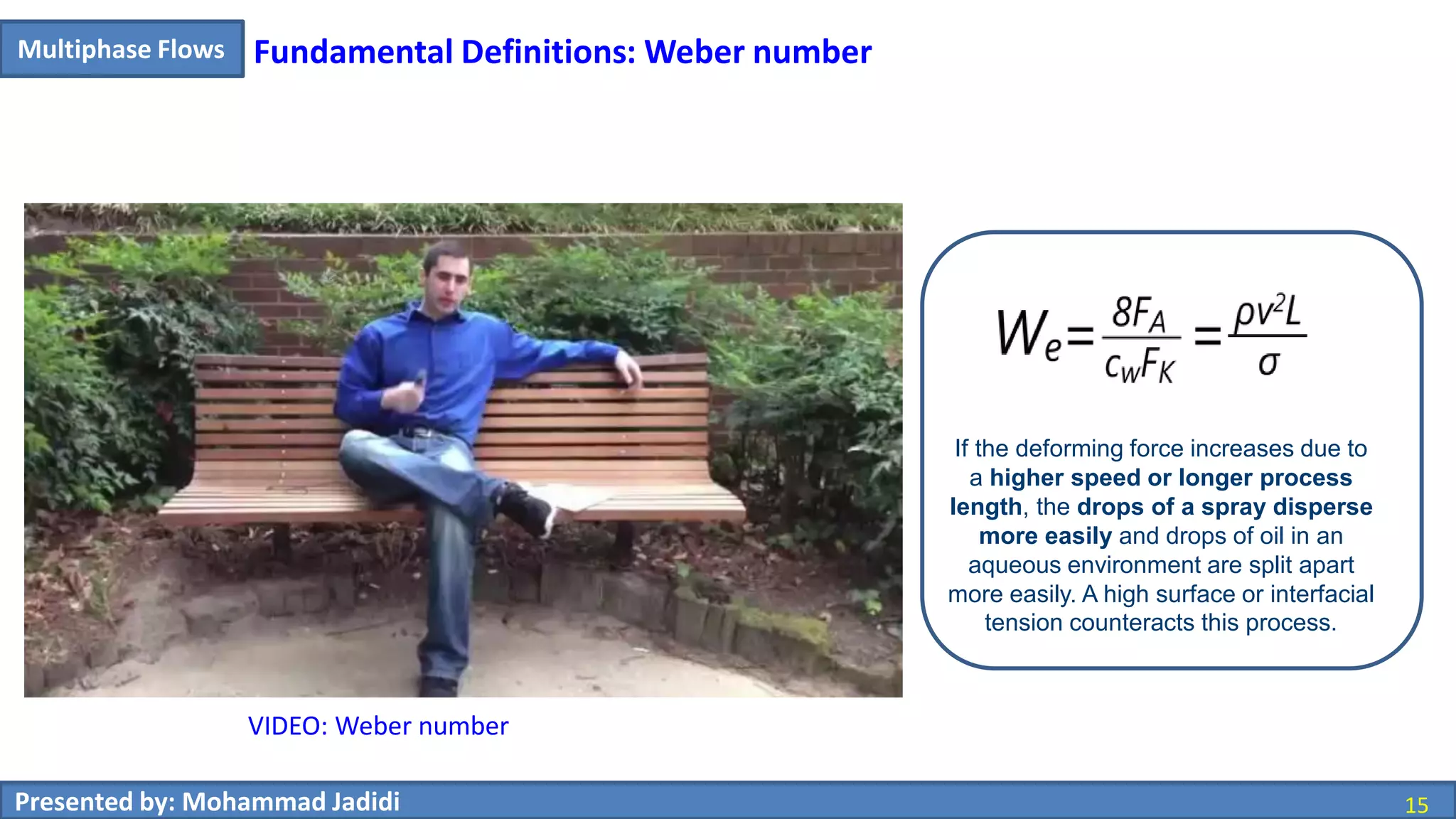
Introduction to Weber number and its effects on fluid dynamics, influencing droplet dispersion in multiphase flows.
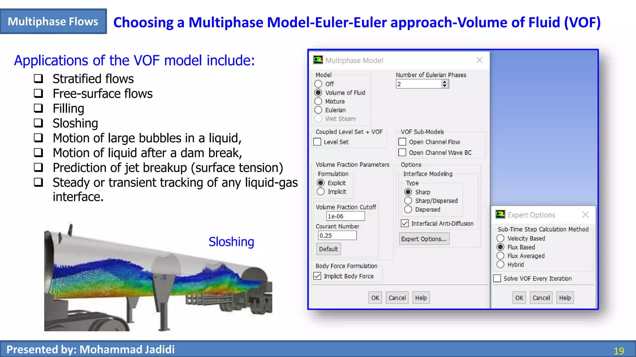
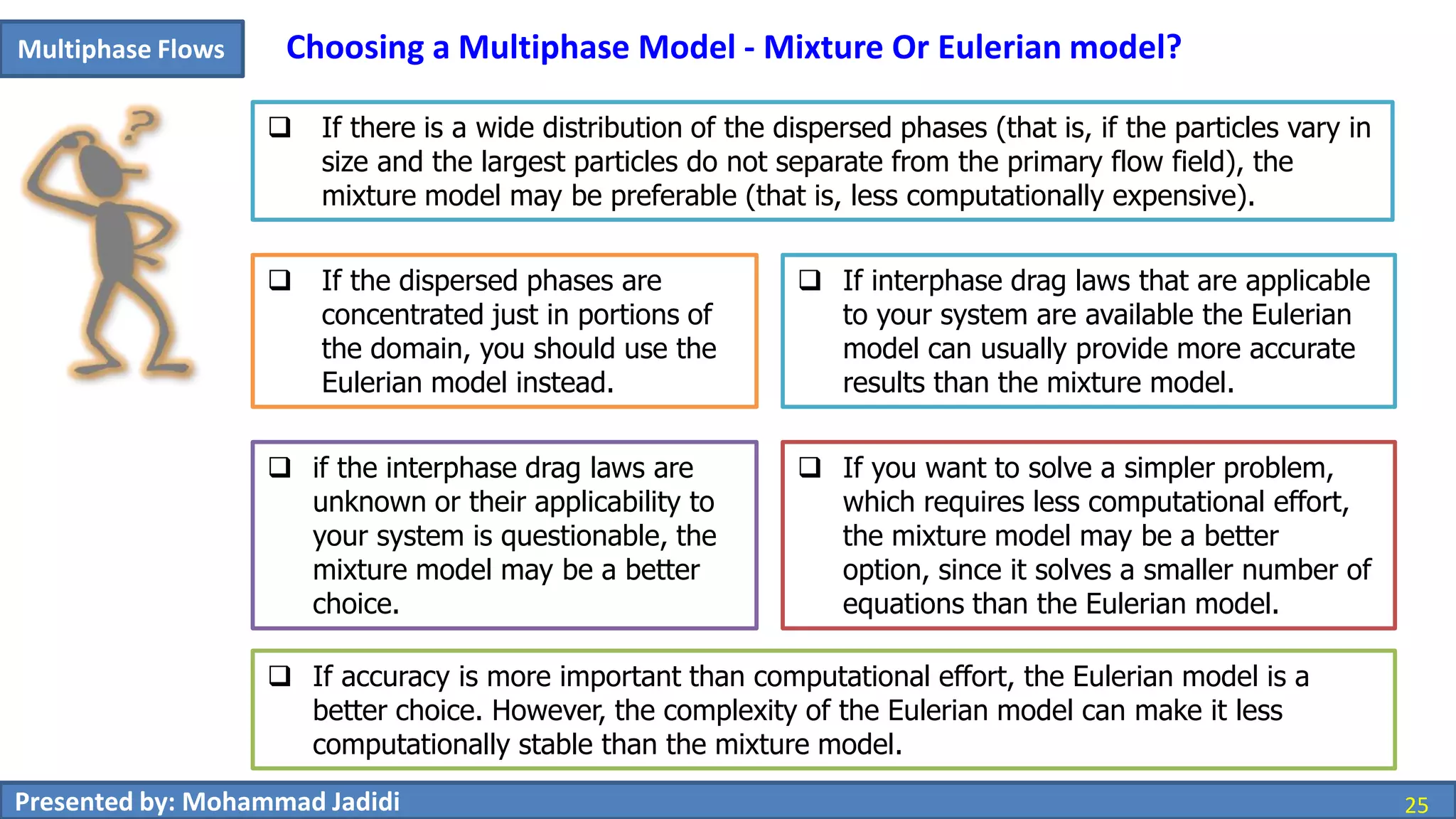
A guide to choosing appropriate multiphase models based on specific flow regimes, loading conditions, and accuracy requirements.
Summary of findings and acknowledgement of the audience, leading into the next part of the presentation.