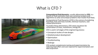
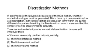
Computational Fluid Dynamics (CFD)

Computational Fluid
Dynamics
Submitted by
Khusro Kamaluddin
ME-1 IVth Year
Submitted to
Mr. Ravi Goel
Department of Mechanical Engineering Quantum School of
Technology Roorkee - 247667(.K.)

What is CFD ?
Computational fluid dynamics, usually abbreviated as CFD, is a
branch of fluid mechanics that uses numerical analysis and
algorithms to solve and analyze problems that involve fluid flows.
Computational Fluid Dynamics (CFD) is the science of predicting
fluid flow, heat and mass transfer, chemical reactions, and
related phenomena.
To predict these phenomena, CFD solves equations for
conservation of mass, momentum, energy etc..
CFD is used in all stages of the engineering process:
• Conceptual studies of new designs
• Detailed product development
• Optimization
• Troubleshooting
• Redesign
CFD analysis complements testing and experimentation by
reducing total effort and cost required for experimentation and
data acquisition

Previously Available Methods
Historically there were two broad methodologies for solving fluid flow
problems :
1. Analytical Fluid Dynamics (AFD)
2. Experimental Fluid Dynamics (EFD)

Analytical Fluid Dynamics (AFD) : The exact solutions of fluid flow
problems were found by applying first principles of fluid dynamics
along with mathematical modelling of the entire fluid domain by
various mathematical techniques. But even a little increase in fluid
model the mathematical exponentially increased. Further it is
practically impossible to mathematically model complicated fluid flow
situations.
Weakness : Cannot be independently verified and very difficult for
complex flow.

Experimental Fluid Dynamics (EFD) : The flow problem is solved by
making a model of the domain and the measurable flow properties are
measured using various measurement techniques(such as hot wire
anemometry, Acoustics Doppler Current Profiler) and then other
properties can be calculated using imperial relationships.
Moreover Experimental Fluid Dynamics was used to verify the results
obtained from Analytical Fluid Dynamics.
Weakness : loss of (significant/insignificant)similitude in case of
extremely large and small domains and error in measurements.

Birth of CFD
With the advance of computational capabilities and numerical
techniques in 1950s various alternate methods to solve fluid flow
problems were found under the common name CFD.
This involved :
Constructing a
fluid domain to
be analyzed.
Applying
Suitable
Boundary
Conditions.
Breaking the
domain into
finite small
elements using
discretization
methods.
Generating
differential
equations for
each of the
generated
element.
Converting of
each of the
differential
equation into a
linear equation
using
numerical
techniques.
Using the
Computational
Capabilities to
solve these
equations in an
iterative
fashion.
Bringing
together all
the elements
properties and
use suitable
interpolation
for the final
results.

Is CFD an Independent Technique ?
Although it seams that every thing we need to
analyze a fluid domain is already in there. But it is
not the case. It is just a simulation and the
authenticity of the simulation cannot be verified
unless it is compared with the real world.
Experimental Fluid Dynamics is used to test the
validity of a CFD simulation and is more or less an
approval that the CFD model is correct and can
further be applied to similar situations without even
getting verified.
NO

Is CFD an Independent Technique ?
CFD is indeed a very powerful TOOL if used wisely.
• It can be used to study fluid flows in visually
obstructed situations(ex. Flows in nuclear reactor,
combustion chamber etc. )
• It can be used to short list experiments to find the
best options that can be the solution.
• To help get hands on more comprehensive results
in the fluid domain that couldn’t have been
possible with experiments alone.
TOOL

Turbulence Models
• A turbulence model is a computational procedure to close the system of mean flow
equations.
• For most engineering applications it is unnecessary to resolve the details of the turbulent
fluctuations.
• Turbulence models allow the calculation of the mean flow without first calculating the
full time-dependent flow field.
• We only need to know how turbulence affected the mean flow.
• In particular we need expressions for the Reynolds stresses.
• For a turbulence model to be useful it:
1. must have wide applicability
2. be accurate
3. simple
4. economical to run.

Turbulence Models
Common turbulence models :
Classical models. Based on Reynolds Averaged Navier-Stokes (RANS)
equations (time averaged):
1. Zero equation model: mixing length model.
2. One equation model: Spalart-Almaras.
3. Two equation models: k- ε style models (standard, RNG, realizable), k- ω
model.
4. Seven equation model: Reynolds stress model.
The number of equations denotes the number of additional PDEs that are
being solved.

Discretization Methods
In order to solve the governing equations of the fluid motion, first their
numerical analogue must be generated. This is done by a process referred to
as discretization. In the discretization process, each term within the partial
differential equation describing the flow is written in such a manner that the
computer can be programmed to calculate.
There are various techniques for numerical discretization. Here we will
introduce three
of the most commonly used techniques, namely:
(1) The finite difference method
(2) The finite element method
(3) The finite volume method

The Finite Volume Method
The finite volume method is currently the
most popular method in CFD.
Generally, the finite volume method is a
special case of finite element. A typical finite
volume, or cell, is shown. In this figure the
centroid of the volume, point P, is the
reference point at which we want to
discretize the partial differential equation.

The Finite Volume Method
The above method is also referred to as the Cell
Centered (CC) Method, where the flow variables are
allocated at the center of the computational cell. The CC
variable arrangement is the most popular, since it leads
to considerably simpler implementations than other
arrangements. On the other hand, the CC arrangement is
more susceptible to truncation errors, when the mesh
departs from uniform rectangles.
Traditionally the finite volume methods have used
regular grids for the efficiency of the computations.
However, recently, irregular grids have become more
popular for simulating flows in complex geometries.
Obviously, the computational effort is more when
irregular grids are used, since the algorithm should use a
table to lookup the geometrical relationships between
the volumes or element faces. This involves.

Steps involved in CFD
CFD codes are structured around the numerical algorithms that can
tackle fluid flow problems. In order to provide easy access to their
solving power all commercial CFD packages include sophisticated user
interfaces to input problem parameters and to examine the results.
Hence all codes contain three main elements:
1. Pre-processor
2. Solver
3. Post-processor

Pre-processor
Pre-processing consists of the input of a flow problem to a CFD program by means
of an operator-friendly interface and the subsequent transformation of this input
into a form suitable for use by the solver. The user activities at the pre-processing
stage involve:
• Definition of the geometry of the region of interest: the computational domain
• Grid generation – the sub-division of the domain into a number of smaller, non-
overlapping sub-domains: a grid (or mesh) of cells (or control volumes or elements)
• Selection of the physical and chemical phenomena that need to be modelled
• Definition of fluid properties
• Specification of appropriate boundary conditions at cells which coincide with or
touch the domain boundary

Definition of Geometry
Step 1: Define your modelling Goals

Step 2: Identify the domain you will model

Step 3: Create a solid model for the domain

Step 4: Design and create the mesh

Meshing
In computational solutions of partial differential equations, meshing is a discrete representation of the geometry that is
involved in the problem. Essentially, it partitions space into elements (or cells or zones) over which the equations can be
approximated. Zone boundaries can be free to create computationally best shaped zones, or they can be fixed to represent
internal or external boundaries within a model.
The mesh quality can be conclusively determined based on the following factors.
• Rate of convergence
The greater the rate of convergence, the better the mesh quality. It means that the correct solution has been achieved
faster. An inferior mesh quality may leave out certain important phenomena such as the boundary layer that occurs in fluid
flow. In this case the solution may not converge or the rate of convergence will be impaired.
• Solution accuracy
A better mesh quality provides a more accurate solution. For example, one can refine the mesh at certain areas of the
geometry where the gradients are high, thus increasing the fidelity of solutions in the region. Also, this means that if a
mesh is not sufficiently refined then the accuracy of the solution is more limited. Thus, mesh quality is dictated by the
required accuracy.
• CPU time required
CPU time is a necessary yet undesirable factor. For a highly refined mesh, where the number of cells per unit area is
maximum, the CPU time required will be relatively large. Time will generally be proportional to the number of elements.

Meshing
Common cell shapes :
1. Two Dimensional :
There are two types of two-dimensional cell shapes that are commonly used.
These are the triangle and the quadrilateral.
Computationally poor elements will have sharp internal angles or short edges
or both.
• Triangle
This cell shape consists of 3 sides and is one of the simplest types of mesh. A
triangular surface mesh is always quick and easy to create. It is most common
in unstructured grids.
• Quadrilateral
This cell shape is a basic 4 sided one as shown in the figure. It is most
common in structured grids.
Quadrilateral elements are usually excluded from being or becoming concave.

Meshing
Common cell shapes :
2. Three Dimensional :
The basic 3-dimensional element are the tetrahedron, quadrilateral pyramid, triangular prism, and hexahedron. They
all have triangular and quadrilateral faces.
Extruded 2-dimensional models may be represented entirely by prisms and hexahedra as extruded triangles and
quadrilaterals.
In general, quadrilateral faces in 3-dimensions may not be perfectly planar. A nonplanar quadrilateral face can be
considered a thin tetrahedral volume that is shared by two neighboring elements.
Tetrahedron
A tetrahedron has 4 vertices, 6 edges, and is bounded by 4 triangular faces. In most cases a tetrahedral volume mesh
can be generated automatically.
Pyramid
A quadrilaterally-based pyramid has 5 vertices, 8 edges, bounded by 4 triangular and 1 quadrilateral face. These are
effectively used as transition elements between square and triangular faced elements and other in hybrid meshes
and grids.
Triangular prism
A triangular prism has 6 vertices, 9 edges, bounded by 2 triangular and 3 quadrilateral faces. The advantage with this
type of layer is that it resolves boundary layer efficiently.
Hexahedron
A hexahedron, a topological cube, has 8 vertices, 12 edges, bounded by 6 quadrilateral faces. It is also called a hex or
a brick.For the same cell amount, the accuracy of solutions in hexahedral meshes is the highest.
The pyramid and triangular prism zones can be considered computationally as degenerate hexahedrons, where some
edges have been reduced to zero. Other degenate forms of a hexahedron may also be represented.

Meshing
Classification of grids :
• Structured grids
Structured grids are identified by regular connectivity. The possible element choices
are quadrilateral in 2D and hexahedra in 3D. This model is highly space efficient, i.e.
since the neighborhood relationships are defined by storage arrangement. Some
other advantages of structured grid over unstructured are better convergence and
higher resolution.
• Unstructured grids
An unstructured grid is identified by irregular connectivity. It cannot easily be
expressed as a two-dimensional or three-dimensional array in computer memory.
This allows for any possible element that a solver might be able to use. Compared to
structured meshes, this model can be highly space inefficient since it calls for explicit
storage of neighborhood relationships. These grids typically employ triangles in 2D
and tetrahedra in 3D.
• Hybrid/multizone grids
A hybrid grid contains a mixture of structured portions and unstructured portions. It
integrates the structured meshes and the unstructured meshes in an efficient
manner. Those parts of the geometry that are regular can have structured grids and
those that are complex can have unstructured grids. These grids can be non-
conformal which means that grid lines don’t need to match at block boundaries.

Meshing
Mesh – Hexahedron(Hex)

Meshing
Mesh – Tetrahedron (Tet)

Meshing
Mesh – Tetrahedral (Prism)

Meshing
Mesh – Recommendation
• 1st Option -> Hex grid
– Best accuracy and numerical efficiency
– Time and effort manageable?
• 2nd Option -> Tet/hex/pyramid grid
– Hex near walls & shear layers
– Developing technology …
• 3rd Option -> Tet/prism grid
– High degree of automation
– Quality (prism/tet transition, …)
• 4th Option -> Tet grid
– Shear layer resolution?

Best Practices-Meshing
Grid must be able to capture
important physics:
– Boundary layers
– Heat transfer
– Wakes, shock
– Flow gradients

Mesh Quality

Mesh Quality
It is very important to keep in mind that CDF
utilizes Finite Volume Method as it
discretization method.
Finite Volume Method is a Cell Centric (CC)
method and results are catastrophic for
irregular cell shapes(if not very small in
size).Thus it is always advisable to keep the
meshing uniform. But to capture various
phenomena the mesh density has to be
varied.
For this very reason it is strongly
recommended that the variation of the mesh
size should not be abrupt but smooth.

Boundary Conditions
Available Boundary condition types :

Boundary Conditions
Symmetry Boundary Condition

Pre-processor
The solution to a flow problem (velocity, pressure,
temperature etc.) is defined at nodes inside each cell. The
accuracy of a CFD solution is governed by the number of
cells in the grid. In general, the larger the number of cells,
the better the solution accuracy. Both the accuracy of a
solution and its cost in terms of necessary computer
hardware and calculation time are dependent on the
fineness of the grid. Optimal meshes are often non-uniform:
finer in areas where large variations occur from point to
point and coarser in regions with relatively little change.
Efforts are under way to develop CFD codes with a (self-
)adaptive meshing capability. Ultimately such programs will
automatically refine the grid in areas of rapid variations. A
substantial amount of basic development work still needs to
be done before these techniques are robust enough to be
incorporated into commercial CFD codes. At present it is still
up to the skills of the CFD user to design a grid that is a
suitable compromise between desired accuracy and solution
cost.
Over 50% of the time spent in industry on a CFD project is
devoted to the definition of the domain geometry and grid
generation

Solver
There are three distinct streams of numerical solution techniques:
finite difference, finite element and spectral methods. We shall be
solely concerned with the finite volume method, a special finite
difference formulation that is central to the most well-established CFD
codes: CFX/ANSYS, FLUENT, PHOENICS and STAR-CD. In outline the
numerical algorithm consists of the following steps:
• Integration of the governing equations of fluid flow over all the
(finite) control volumes of the domain
• Discretisation – conversion of the resulting integral equations into a
system of algebraic equations
• Solution of the algebraic equations by an iterative method

Solver
The first step, the control volume integration, distinguishes the finite volume method from all
other CFD techniques.
The resulting statements express the (exact) conservation of relevant properties for each finite
size cell. This clear relationship between the numerical algorithm and the underlying physical
conservation principle forms one of the main attractions of the finite volume method and makes
its concepts much more simple to understand by engineers than the finite element and spectral
methods. The conservation of a general flow variable φ, e.g. a velocity component or enthalpy,
within a finite control volume can be expressed as a balance between the various processes
tending to increase or decrease it. In words we have:
CFD codes contain discretisation techniques suitable for the treatment of the key transport
phenomena, convection (transport due to fluid flow) and diffusion (transport due to variations of
φ from point to point) as well as for the source terms (associated with the creation or destruction
of φ) and the rate of change with respect to time. The underlying physical phenomena are
complex and non-linear so an iterative solution approach is required.

Solver
Solution Procedure Overview :

Solver
Pressure-based Solver (PBS) :

Solver
Density-based Solver (DBS) :

Post-processor
As in pre-processing, a huge amount of development
work has recently taken place in the post-processing
field. Due to the increased popularity of engineering
workstations, many of which have outstanding graphics
capabilities, the leading CFD packages are now
equipped with versatile data visualization tools. These
include:
• Domain geometry and grid display
• Vector plots
• Line and shaded contour plots
• 2D and 3D surface plots
• Particle tracking
• View manipulation (translation, rotation, scaling etc.)
• Colour PostScript outpu

Post-processor
As in pre-processing, a huge amount of development
work has recently taken place in the post-processing
field. Due to the increased popularity of engineering
workstations, many of which have outstanding graphics
capabilities, the leading CFD packages are now
equipped with versatile data visualization tools. These
include:
• Domain geometry and grid display
• Vector plots
• Line and shaded contour plots
• 2D and 3D surface plots
• Particle tracking
• View manipulation (translation, rotation, scaling etc.)
• Color PostScript output

Biblography
1. Fluent User ‘s Guide (Online)
2. F M White “Fluid Mechanics” 7th Edition Mc Graw Hill
3. H. Versteeg, W. Malalasekra-An Introduction to Computational Fluid
Dynamics_ The Finite Volume Method (2nd Edition) -Prentice Hall
(2007)
4. Date A. W.-Introduction to Computational Fluid Dynamics (2005)
5. Anderson, Computational Fluid Dynamics With Basics and Applications
Mc Graw Hill
6. Kundu Cohen Dowling Fluid Mechanics 5th Edition Academic Press

Computational Fluid Dynamics (CFD)

More Related Content

What's hot

Viewers also liked

Similar to Computational Fluid Dynamics (CFD)

More from Khusro Kamaluddin

Recently uploaded

Computational Fluid Dynamics (CFD)