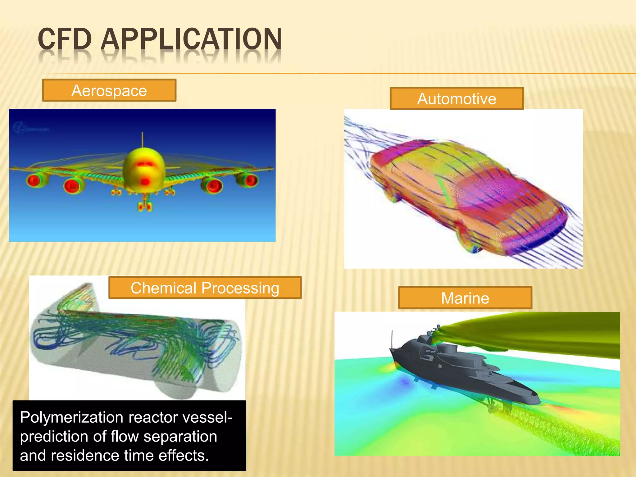
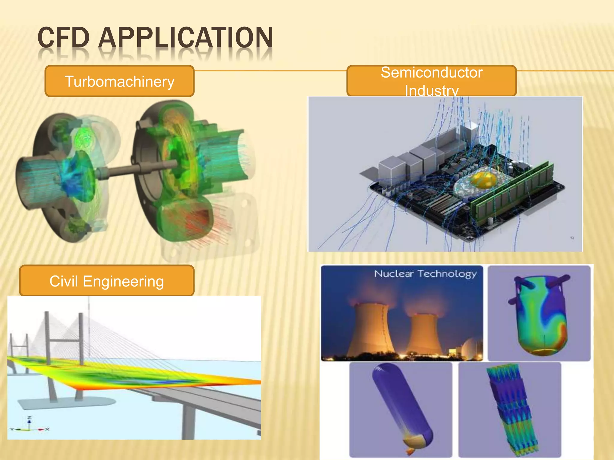
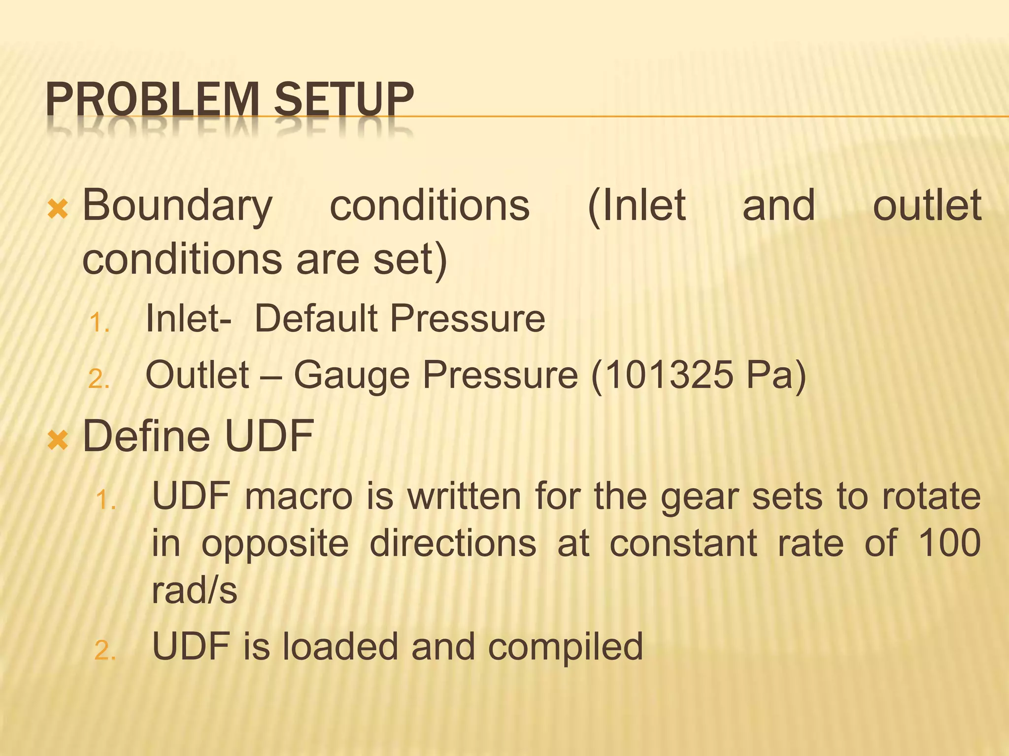
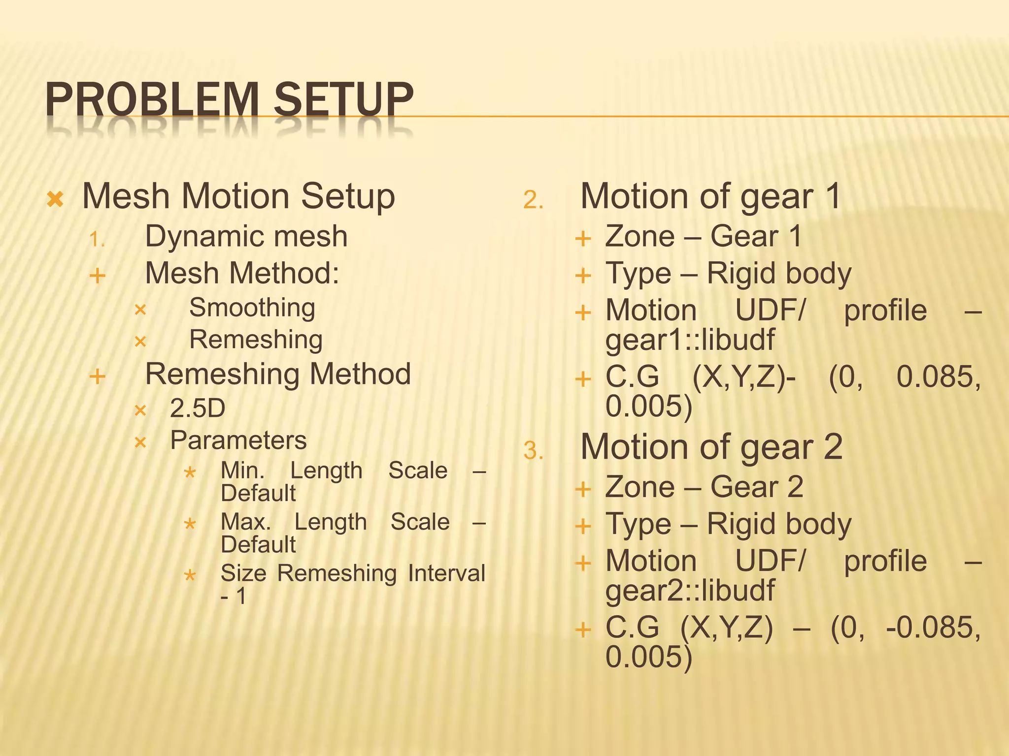
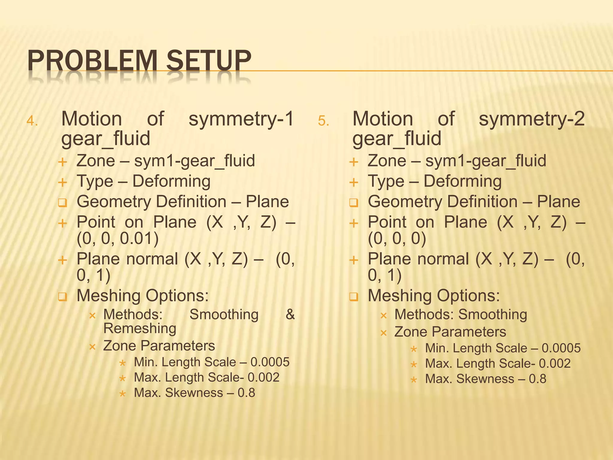
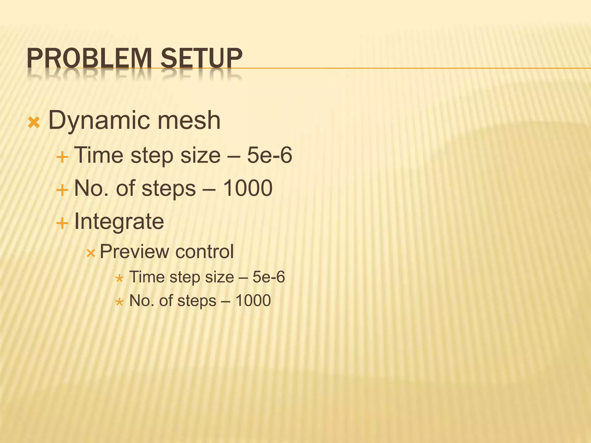
ANALYSIS OF GEAR PUMP USING
ANSYS FLUENT
SAVANI BHAVIK B.
INTRODUCTION
 What is CFD?
CFD: A methodology for obtaining a discrete
solution of real world fluid flow problems.
Discrete solution: Solution is obtained at a
finite collection of space points and at discrete
time levels
CFD IN A NUTSHELL
 Solving the governing equation of fluid by using computational
methods under various physical conditions (e.g. heat transfer,
radiation, electromagnetic field, nuclear reaction…etc.) to study
different phenomena encountered in the numerous branches of
physical science.
CFD APPLICATION
Aerospace
Automotive
Chemical Processing
Polymerization reactor vessel-
prediction of flow separation
and residence time effects.
Marine
CFD APPLICATION
Turbomachinery
Semiconductor
Industry
Civil Engineering
BUILDING BLOCKS
Geometry & grid
generation module
Problem setting
module
Solution Module
Visualization
Module
What to: Presume
• Boundary / initial conditions
• Physical models
& what to: Neglect
• Physical phenomena (i.e. heat transfer, chemical
reaction…etc)
• Properties (i.e. Compressibility, real gas…etc)
& what to : Calculate
• Unknowns
• Relationships between field variable
Solution methods & algorithms
• Spatial / temporal discretization
schemes
• Convergence criterion
• Interpolation methods
METHODOLOGY
 During Preprocessing
 The geometry of the problem is defined
 The volume occupied by the fluid is divided into discrete cells.
The mesh may be uniform or non-uniform
 The physical modelling is defined – for eg. The equation of
motion + enthalpy + radiation + species conservation
 Boundary conditions are defined. This involves specifying the
fluid behavior and properties at the boundaries of the problem.
For transient problems, the initial conditions are also defined
 The simulation is started and the equation are solved
iteratively as a steady-state or transient
 Finally a postprocessor is used for the analysis and
visualization of the resulting solution.
FINITE VOLUME METHOD USED IN
DISCRETIZATION
 The finite volume method (FVM) is a common approach used in CFD
codes, as it has an advantage in memory usage and solution speed,
especially for large problems, high Reynolds number turbulent flows,
and source term dominated flows (like combustion).
 In this method the governing partial differential equations are recast in
the conservative form and then solved over a discrete control volumes
and thus guarantees the conservation of fluxes through a particular
control volume.
 Here Q is the vector of conserved variables, F is the vector of
fluxes V is the volume of the control volume element, and A is the
surface area of the control volume element. The finite volume
equation yields governing equations in the form:
FINITE ELEMENT METHOD
 The finite element method (FEM) is used in
structural analysis of solids, but is also
applicable to fluids.
 It is much more stable than the finite volume
approach. However, it can require more
memory and has slower solution than the
FVM.
FINITE DIFFERENCE METHOD
 The finite difference method (FDM) has
historical importance and is simple to
program.
 It is currently only used in few specialized
codes, which handle complex geometry with
high accuracy and efficiency by using
embedded boundaries or overlapping grids
(with the solution interpolated across each
grid).
PURPOSE OF PRESENTATION
GEAR PUMP
 A gear pump uses
the meshing of gears
to pump fluid by
displacement.
 There are two main
variation: external
gear pump and
internal gear pump
 Gear pump are
positive displacement
meaning they pump a
constant amount of
fluid for each
revolution.
THEORY OF OPERATION
 As the gears rotate they separate on the intake
side of the pump, creating a void and suction
which is filled by fluid. The fluid is carried by the
gears to the discharge side of the pump, where
the meshing of the gears displaces the fluid.
 Mechanical clearances are small, which
prevents the fluid from leaking backwards.
 Rigid design of the gears and houses allow for
very high pressures and the ability to pump
highly viscous fluids.
Internal Gear
Pump
External
Gear Pump
PROCESS IN SOLVING PROBLEM
 Set up a problem using the 2.5D dynamic re-
meshing model.
 Specify dynamic mesh modeling parameters.
 Specify a rigid body motion zone.
 Specify a deforming zone.
 Use prescribed motion UDF macro.
 Perform the calculation with residual plotting.
 Post process using CFD-Post.
PROBLEM STATEMENT
 The current setup is an external gear pump
which uses two external spur gears.
 Gears rotate at constant rate of 100 rad/s.
 Fluid- oil (Density- 844 kg/m3 & Viscosity –
0.02549 kg/m-s)
 Mass flow rate of fluid in and out of the pump
is of interest.
PROBLEM SCHEMATIC
MESH
PROBLEM SETUP
 General setting- Solver
1. Type- pressure-Based
2. Velocity Formulation- Absolute
3. Time – Transient
 Models- Viscous - Realizable k-epsilon with
standard wall function
PROBLEM SETUP
 Material
1. Material – oil
2. Density -844 kg/m3
3. Viscosity – 0.02549 kg /m-s
 Cell Zone conditions
1. Each cell zone, select material as oil
PROBLEM SETUP
 Boundary conditions (Inlet and outlet
conditions are set)
1. Inlet- Default Pressure
2. Outlet – Gauge Pressure (101325 Pa)
 Define UDF
1. UDF macro is written for the gear sets to rotate
in opposite directions at constant rate of 100
rad/s
2. UDF is loaded and compiled
PROBLEM SETUP
 Mesh Motion Setup
1. Dynamic mesh
 Mesh Method:
 Smoothing
 Remeshing
 Remeshing Method
 2.5D
 Parameters
 Min. Length Scale –
Default
 Max. Length Scale –
Default
 Size Remeshing Interval
- 1
2. Motion of gear 1
 Zone – Gear 1
 Type – Rigid body
 Motion UDF/ profile –
gear1::libudf
 C.G (X,Y,Z)- (0, 0.085,
0.005)
3. Motion of gear 2
 Zone – Gear 2
 Type – Rigid body
 Motion UDF/ profile –
gear2::libudf
 C.G (X,Y,Z) – (0, -0.085,
0.005)
PROBLEM SETUP
4. Motion of symmetry-1
gear_fluid
 Zone – sym1-gear_fluid
 Type – Deforming
 Geometry Definition – Plane
 Point on Plane (X ,Y, Z) –
(0, 0, 0.01)
 Plane normal (X ,Y, Z) – (0,
0, 1)
 Meshing Options:
 Methods: Smoothing &
Remeshing
 Zone Parameters
 Min. Length Scale – 0.0005
 Max. Length Scale- 0.002
 Max. Skewness – 0.8
5. Motion of symmetry-2
gear_fluid
 Zone – sym1-gear_fluid
 Type – Deforming
 Geometry Definition – Plane
 Point on Plane (X ,Y, Z) –
(0, 0, 0)
 Plane normal (X ,Y, Z) – (0,
0, 1)
 Meshing Options:
 Methods: Smoothing
 Zone Parameters
 Min. Length Scale – 0.0005
 Max. Length Scale- 0.002
 Max. Skewness – 0.8
PROBLEM SETUP
 Dynamic mesh
 Time step size – 5e-6
 No. of steps – 1000
 Integrate
 Preview control
 Time step size – 5e-6
 No. of steps – 1000
SOLUTION
 Solution methods
 Retain defaults
 Solution controls
 Relaxation factor of
pressure- 0.4
 Momentum – 0.5
 Turbulent K.E – 0.7
 Turbulent dissipation rate
– 0.7
 Turbulent viscosity – 0.75
 Solution initialization
 TKE – 0.1
 Gauge pressure – 101325
Pa
 Initialize the solution
 Run Solution (Run
calculation for 150 time
steps)
 Time step size- 5e-6
 No. of time steps – 3000
 Max iterations / time step –
40
 Calculate
POSTPROCESSING
Velocity
Contour
Pressure
Contour
CONCLUSION
 The accuracy of the computed flow rate for a
given model increases as the outlet pressure
decreases.
CFD Introduction using Ansys Fluent

CFD Introduction using Ansys Fluent

  • 1.
    ANALYSIS OF GEARPUMP USING ANSYS FLUENT SAVANI BHAVIK B.
  • 2.
    INTRODUCTION  What isCFD? CFD: A methodology for obtaining a discrete solution of real world fluid flow problems. Discrete solution: Solution is obtained at a finite collection of space points and at discrete time levels
  • 3.
    CFD IN ANUTSHELL  Solving the governing equation of fluid by using computational methods under various physical conditions (e.g. heat transfer, radiation, electromagnetic field, nuclear reaction…etc.) to study different phenomena encountered in the numerous branches of physical science.
  • 4.
    CFD APPLICATION Aerospace Automotive Chemical Processing Polymerizationreactor vessel- prediction of flow separation and residence time effects. Marine
  • 5.
  • 6.
    BUILDING BLOCKS Geometry &grid generation module Problem setting module Solution Module Visualization Module What to: Presume • Boundary / initial conditions • Physical models & what to: Neglect • Physical phenomena (i.e. heat transfer, chemical reaction…etc) • Properties (i.e. Compressibility, real gas…etc) & what to : Calculate • Unknowns • Relationships between field variable Solution methods & algorithms • Spatial / temporal discretization schemes • Convergence criterion • Interpolation methods
  • 7.
    METHODOLOGY  During Preprocessing The geometry of the problem is defined  The volume occupied by the fluid is divided into discrete cells. The mesh may be uniform or non-uniform  The physical modelling is defined – for eg. The equation of motion + enthalpy + radiation + species conservation  Boundary conditions are defined. This involves specifying the fluid behavior and properties at the boundaries of the problem. For transient problems, the initial conditions are also defined  The simulation is started and the equation are solved iteratively as a steady-state or transient  Finally a postprocessor is used for the analysis and visualization of the resulting solution.
  • 8.
    FINITE VOLUME METHODUSED IN DISCRETIZATION  The finite volume method (FVM) is a common approach used in CFD codes, as it has an advantage in memory usage and solution speed, especially for large problems, high Reynolds number turbulent flows, and source term dominated flows (like combustion).  In this method the governing partial differential equations are recast in the conservative form and then solved over a discrete control volumes and thus guarantees the conservation of fluxes through a particular control volume.  Here Q is the vector of conserved variables, F is the vector of fluxes V is the volume of the control volume element, and A is the surface area of the control volume element. The finite volume equation yields governing equations in the form:
  • 9.
    FINITE ELEMENT METHOD The finite element method (FEM) is used in structural analysis of solids, but is also applicable to fluids.  It is much more stable than the finite volume approach. However, it can require more memory and has slower solution than the FVM.
  • 10.
    FINITE DIFFERENCE METHOD The finite difference method (FDM) has historical importance and is simple to program.  It is currently only used in few specialized codes, which handle complex geometry with high accuracy and efficiency by using embedded boundaries or overlapping grids (with the solution interpolated across each grid).
  • 11.
    PURPOSE OF PRESENTATION GEARPUMP  A gear pump uses the meshing of gears to pump fluid by displacement.  There are two main variation: external gear pump and internal gear pump  Gear pump are positive displacement meaning they pump a constant amount of fluid for each revolution.
  • 12.
    THEORY OF OPERATION As the gears rotate they separate on the intake side of the pump, creating a void and suction which is filled by fluid. The fluid is carried by the gears to the discharge side of the pump, where the meshing of the gears displaces the fluid.  Mechanical clearances are small, which prevents the fluid from leaking backwards.  Rigid design of the gears and houses allow for very high pressures and the ability to pump highly viscous fluids.
  • 13.
  • 14.
    PROCESS IN SOLVINGPROBLEM  Set up a problem using the 2.5D dynamic re- meshing model.  Specify dynamic mesh modeling parameters.  Specify a rigid body motion zone.  Specify a deforming zone.  Use prescribed motion UDF macro.  Perform the calculation with residual plotting.  Post process using CFD-Post.
  • 15.
    PROBLEM STATEMENT  Thecurrent setup is an external gear pump which uses two external spur gears.  Gears rotate at constant rate of 100 rad/s.  Fluid- oil (Density- 844 kg/m3 & Viscosity – 0.02549 kg/m-s)  Mass flow rate of fluid in and out of the pump is of interest.
  • 16.
  • 17.
  • 18.
    PROBLEM SETUP  Generalsetting- Solver 1. Type- pressure-Based 2. Velocity Formulation- Absolute 3. Time – Transient  Models- Viscous - Realizable k-epsilon with standard wall function
  • 19.
    PROBLEM SETUP  Material 1.Material – oil 2. Density -844 kg/m3 3. Viscosity – 0.02549 kg /m-s  Cell Zone conditions 1. Each cell zone, select material as oil
  • 20.
    PROBLEM SETUP  Boundaryconditions (Inlet and outlet conditions are set) 1. Inlet- Default Pressure 2. Outlet – Gauge Pressure (101325 Pa)  Define UDF 1. UDF macro is written for the gear sets to rotate in opposite directions at constant rate of 100 rad/s 2. UDF is loaded and compiled
  • 21.
    PROBLEM SETUP  MeshMotion Setup 1. Dynamic mesh  Mesh Method:  Smoothing  Remeshing  Remeshing Method  2.5D  Parameters  Min. Length Scale – Default  Max. Length Scale – Default  Size Remeshing Interval - 1 2. Motion of gear 1  Zone – Gear 1  Type – Rigid body  Motion UDF/ profile – gear1::libudf  C.G (X,Y,Z)- (0, 0.085, 0.005) 3. Motion of gear 2  Zone – Gear 2  Type – Rigid body  Motion UDF/ profile – gear2::libudf  C.G (X,Y,Z) – (0, -0.085, 0.005)
  • 22.
    PROBLEM SETUP 4. Motionof symmetry-1 gear_fluid  Zone – sym1-gear_fluid  Type – Deforming  Geometry Definition – Plane  Point on Plane (X ,Y, Z) – (0, 0, 0.01)  Plane normal (X ,Y, Z) – (0, 0, 1)  Meshing Options:  Methods: Smoothing & Remeshing  Zone Parameters  Min. Length Scale – 0.0005  Max. Length Scale- 0.002  Max. Skewness – 0.8 5. Motion of symmetry-2 gear_fluid  Zone – sym1-gear_fluid  Type – Deforming  Geometry Definition – Plane  Point on Plane (X ,Y, Z) – (0, 0, 0)  Plane normal (X ,Y, Z) – (0, 0, 1)  Meshing Options:  Methods: Smoothing  Zone Parameters  Min. Length Scale – 0.0005  Max. Length Scale- 0.002  Max. Skewness – 0.8
  • 23.
    PROBLEM SETUP  Dynamicmesh  Time step size – 5e-6  No. of steps – 1000  Integrate  Preview control  Time step size – 5e-6  No. of steps – 1000
  • 24.
    SOLUTION  Solution methods Retain defaults  Solution controls  Relaxation factor of pressure- 0.4  Momentum – 0.5  Turbulent K.E – 0.7  Turbulent dissipation rate – 0.7  Turbulent viscosity – 0.75  Solution initialization  TKE – 0.1  Gauge pressure – 101325 Pa  Initialize the solution  Run Solution (Run calculation for 150 time steps)  Time step size- 5e-6  No. of time steps – 3000  Max iterations / time step – 40  Calculate
  • 26.
  • 27.
  • 29.
    CONCLUSION  The accuracyof the computed flow rate for a given model increases as the outlet pressure decreases.

Editor's Notes

  • #9 Eq- Navier stroke’s , mass and energy conservation equations. For this We begin with the incompressible form of the momentum equation and then the equation is integrated over the control volume of a computational cell.
  • #18 The mesh is automatically read into fluent and displayed in the graphics window.
  • #19 Note: problem involving rotation, boundary layers under strong adverse pressure gradients, separation and recirculation, this model shows superior performance over the standard k-epsilon model.
  • #23 Geometry definition parameter are defined to ensure that re- meshing does not cause the mesh to move out of the specified plane.
  • #24 This show the rotation of the zone as a preview. This helps to make sure that the UDF is specifying the motion of the zone correctly
  • #25 Solution controls – this is done because when running the solution it was found that the solution process is more stable with these URFs.