introduction to wall function in turbulence modeling

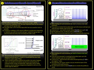
1. Turbulence near the wall - Law of the wall
 Near walls, in the boundary layer, the velocity changes rapidly.
 In turbulence modeling in CFD, the most important zones are the viscous
sub-layer and the log-law layer.
 The buffer layer is the transition layer which we try to avoid as much as
possible.
 Turbulence modeling in CFD requires different considerations depending
on whether you solve the viscous sub-layer, model the log-law layer, or
solve the whole boundary layer (including the buffer zone).
 The use of the non-dimensional velocity (𝑢+) and non-dimensional
distance from the wall (𝑦+) , results in a predictable boundary layer
profile for a wide range of flows.
 Under standard working conditions this profile is the same, however,
under non-equilibrium conditions (production and dissipation of
turbulent kinetic energy not balanced), rough walls, porous media,
buoyancy, viscous heating, strong pressure gradients, and so on, the
profile might be different.
 When dealing with wall turbulence, we need to choose a near-wall
treatment.
 If you want to resolve the boundary layer up to the viscous sub-layer you
need very fine meshes close to the wall.
 In terms of 𝑦+ , you need to cluster at least 6 to 10 layers at 𝒚+< 10.
 But for good accuracy, usually you will use 20 to 30 layers.
 This is the most accurate approach, but it is computationally expensive.
Near-wall treatment and wall functions
 When dealing with wall turbulence, we need to choose a near-wall
treatment.
 If you are not interested in resolving the boundary layer up to the
viscous sub-layer, you can use wall functions.
 In terms of 𝑦+, wall functions will model everything below 𝒚+< 30 or
the target 𝑦+ value.
 This approach use coarser meshes, but you should be aware of the
limitations of the wall functions.
 You will need to cluster at least 5 to 8 layers to resolve the profiles (U
and k)
1 2