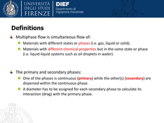
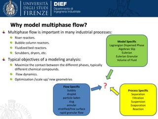
This document discusses modeling and simulation of multiphase flows using computational fluid dynamics (CFD). It begins with definitions of multiphase flow and discusses important types including bubbly, droplet, particle-laden, and annular flows. The document then provides tips on multiphase simulation including choosing appropriate modeling approaches such as Lagrangian, Eulerian, or volume of fluid methods depending on the problem. It concludes with discussions of challenges such as convergence difficulties and appropriate solver settings and techniques to address these challenges.

1. Modeling and simulation of
Mutiphase flows
(CFD tips)
Pouriya Niknam
Supervisor: Dr. Daniele Fiaschi

2. Multiphse flow introduction, definition and types
Tips on multiphase simulation
Outline
2

3. Definitions
Multiphase flow is simultaneous flow of:
Materials with different states or phases (i.e. gas, liquid or solid).
Materials with different chemical properties but in the same state or phase
(i.e. liquid-liquid systems such as oil droplets in water).
The primary and secondary phases:
One of the phases is continuous (primary) while the other(s) (secondary) are
dispersed within the continuous phase.
A diameter has to be assigned for each secondary phase to calculate its
interaction (drag) with the primary phase.

4. Multiphase flow is important in many industrial processes:
Riser reactors.
Bubble column reactors.
Fluidized bed reactors.
Scrubbers, dryers, etc.
Typical objectives of a modeling analysis:
Maximize the contact between the different phases, typically
different chemical compounds.
Flow dynamics.
Optimization /scale up/ new geometries
Why model multiphase flow?
Flow Specific
bubbly
droplet
particle-laden
slug
annular
stratified/free surface
rapid granular flow
Model Specific
Lagrangian Dispersed Phase
Algebraic Slip
Eulerian
Eulerian Granular
Volume of Fluid
Process Specific
Separation
Filtration
Suspension
Evaporation
Reaction
?

5. multiphase or multicomponent?
– Distinguish multiphase and/or multicomponent
• Liquid/Gas or Gas/Liquid
• Gas/Solid
• Liquid/Liquid
– Technically, two immiscible liquids are “multi-fluid”, but are
often referred to as a “multiphase” flow due to their similarity
in behavior
Single component Multi-component
Single phase
Water
Pure nitrogen
Air
H2O+oil emulsions
Multi-phase Steam bubble in H2O
Coal particles in air
Sand particle in H2O
Phase interaction & Species interaction

6. Dispersed/Interfacial
• Flows are also generally categorized by distribution of the components
– “separated” or “interfacial”
• both fluids are more or less contiguous throughout the
domain
– “dispersed”
• One of the fluids is dispersed as non-contiguous
isolated regions within the other (continuous) phase.
• The former is the “dispersed” phase, while the latter
is the “carrier” phase.
• One can now describe/classify the geometry of the
dispersion:
• Size & geometry
• Volume fraction

7. Bubbly Pipe Flow – heat exchangers in power plants, A/C units
Gas-Liquid Flow
Aeration:
-produced by wave action
- used as reactor in chemical processing
- enhanced gas-liquid mass transfer
Ship wakes – detectability
Cavitation – noise, erosion of structures

8. Weather – cloud formation
Biomedical – inhalant drug delivery
Liquid-Gas Flow
Gas-Liquid Flow
Energy production – liquid fuel combustion
Biomedical – inhalant drug delivery

9. Environmental – avalanche, pyroclastic flow, ash
plume, turbidity currents
Gas-Solid Flow
Granular Flow – collision dominated
dynamics; chemical processing

10. Chemical production – mixing and reaction of immiscible liquids
Liquid-Liquid

11. Sediment Transport – pollution, erosion of beaches,
drainage and flood control
Solid-Liquid
Settling/sedimentation, turbidity currents

12. Material processing – generation of particles & composite materials
Energy production – coal combustion
Solid-Gas
Aerosol formation – generation of particles & environmental safety

13. • One-way coupling: Sufficiently dilute such that fluid feels no effect
from presence of particles. Particles move in dynamic response to
fluid motion.
– Fluid phase influences particulate phase via aerodynamic drag and
turbulence transfer.
– No influence of particulate phase on the continous phase.
• Two-way coupling: Enough particles are present such that
momentum exchange between dispersed and carrier phase interfaces
alters dynamics of the carrier phase.
– Fluid phase influences particulate phase via aerodynamic drag and
turbulence transfer.
– Particulate phase reduces mean momentum and turbulent kinetic
energy in fluid phase.
• Four-way coupling: Flow is dense enough that dispersed phase
collisions are significant momentum exchange mechanism
• Includes all two-way coupling.
• Particle-particle collisions create particle pressure and viscous
stresses.
Coupling between phases

14. Empirical correlations.
Lagrangian
Track individual point particles.
Particles do not interact.
Algebraic slip model
Mixture model
Dispersed phase in a continuous phase.
Solve one momentum equation for the mixture.
Neither particle-wall interaction nor particle-particle are taken into account
Two-fluids theory (multi-fluids)
Eulerian-Eulerian models: two co-existing fluids
Solve as many momentum equations as there are phases.
Particle-wall interaction taken into account, particle-particle usually not.
Eulerian-granular model (EGM)
Both particle-wall and particle-particle interaction are taken into account
dispersed phase model (DPM)
Eulerian/Lagrangian
Solve the trajectories of individual objects and their collisions, inside a continuous phase.
Particle-wall interaction always taken into account, particle-particle usually not
Fully resolved and coupled.
Increasedcomplexity
Modeling approach

15. Trajectories of particles/droplets are
computed in a Lagrangian frame.
Exchange (couple) heat, mass, and momentum
with Eulerian frame gas phase.
Discrete phase volume fraction should
preferably be less than 10%.
Mass loading can be large (+100%).
No particle-particle interaction or break up.
Turbulent dispersion modeled by:
Stochastic tracking.
Particle cloud model.
Model particle separation, spray drying,
liquid fuel or coal combustion, etc.
Modeling approach, DPM

16. User must know the characteristics of the flow.
Flow regime, e.g. bubbly flow, slug flow, annular flow, etc.
Laminar or turbulent
Dilute or dense
Secondary phase diameter for drag considerations.
Phases interaction...
Multiphase flow regimes

17. Available Solvers
• There are two kinds of solvers available
in FLUENT – Pressure based and Density
based.
• The pressure-based solvers take
momentum and pressure (or pressure
correction) as the primary variables.
– Pressure-velocity coupling algorithms are
derived by reformatting the continuity
equation
• Two algorithms are available with the
pressure-based solvers:
– Segregated solver – Solves for pressure
correction and momentum sequentially.
– Coupled Solver (PBCS) – Solves pressure
and momentum simultaneously.
Pressure-Based
(segregated)
Density-Based
(coupled)
Solve Mass
Continuity;
Update Velocity
Solve U-Momentum
Solve V-Momentum
Solve W-Momentum
Pressure-Based
(coupled)
Solve Turbulence Equation(s)
Solve Species
Solve Energy
Solve Other Transport Equations as required
Solve Mass
& Momentum
Solve Mass,
Momentum,
Energy,
Species

18. Choosing a Solver
• The pressure-based solver is applicable for a wide range of flow regimes from low
speed incompressible flow to high-speed compressible flow.
– Requires less memory (storage).
– Allows flexibility in the solution procedure.
• The pressure-based coupled solver (PBCS) is applicable for most single phase
flows, and yields superior performance to the standard pressure-based solver.
– Now available for multiphase (Eulerian)
– Requires 1.5–2 times more memory than the segregated solver.
• The density-based coupled solver (DBCS) is applicable when there is a strong
coupling, or interdependence, between density, energy, momentum, and/or
species.
– Examples: High speed compressible flow with combustion, hypersonic flows, shock
interactions.

19. Convergence Difficulties with multiphase
• Numerical instabilities can arise with an ill-posed problem, poor-quality mesh and/or
inappropriate solver settings.
– Exhibited as increasing (diverging) or “stuck” residuals.
– Unconverged results are very misleading!
• Troubleshooting
1. Ensure that the problem is well-posed.
2. Compute an initial solution using a
first-order discretization scheme.
3. For the pressure-based solver, decrease
underrelaxation factors for equations
having convergence problems.
4. For the density-based solver, reduce
the Courant number.
5. Disabling Volume fraction &phase equations
6. Remesh or refine cells which have large
aspect ratio or large skewness.
(Remember that you cannot improve
cell skewness by using mesh adaption!)
Continuity equation convergence
trouble affects convergence of
all equations.

20. Modifying Under-Relaxation Factors
• Under-relaxation factor, α, is included to stabilize the
iterative process for the pressure-based solver
• Use default under-relaxation factors to start a calculation.
• Decreasing under-relaxation
for momentum often aids
convergence.
– Default settings are suitable for a
wide range of problems, you can
reduce the values when necessary.
– Appropriate settings are best learned
from experience!

21. Modifying the Courant Number
• A transient term is included in the density-based solver even for
steady state problems.
– The Courant number defines the
time step size.
• For density-based explicit solver:
– Stability constraints impose a
maximum limit on the Courant
number.
• Cannot be greater than 2
(default value is 1).
• Reduce the Courant number when
having difficulty converging.
• For density-based implicit solver:
– The Courant number is not limited
by stability constraints.
• Default value is 5.

22. Starting from a Previous Solution
• A previously calculated solution can be
used as an initial condition when
changes are made to the case setup.
– Use solution interpolation to
initialize a run (especially
useful for starting fine-mesh cases
when coarse-mesh solutions are
available).
– Once the solution is initialized,
additional iterations always use
the current data set as the starting
point.
– Some suggestions on how to
provide initial conditions for some
actual problems:
Actual Problem Initial Condition
Heat Transfer Isothermal
Natural convection Low Rayleigh number
Turbulence Inviscid (Euler) solution

23. Steady or Unsteady
• Nearly all flows in nature are transient!
– Steady-state assumption is possible if we:
• Ignore unsteady fluctuations
• Employ ensemble/time-averaging to remove unsteadiness (this is
what is done in modeling turbulence)
• In CFD, steady-state methods are preferred
– Lower computational cost
– Easier to postprocess and analyze
• Many applications require resolution of transient flow:
– Aerodynamics (aircraft, land vehicles,etc.) – vortex shedding
– Rotating Machinery – rotor/stator interaction, stall, surge
– Multiphase Flows – free surfaces, bubble dynamics
– Deforming Domains – in-cylinder combustion, store separation
– Unsteady Heat Transfer – transient heating and cooling
– Many more

24. • Typically, compressible analyses are executed in
a transient or pseudo-transient fashion since
the problem is no longer elliptic: downstream
boundary conditions cannot be felt upstream in
a supersonic analysis.
– Pseudo Transient: Use of Inertial Relaxation.
Pseudo Transient
improve multiphase convergency

25. • Symmetry Plane?
• Symmetric geometry does not necessarily mean symmetric flow
– Example: The coanda effect. A jet entering at the center of a symmetrical
duct will tend to flow along one side above a certain Reynolds number
Specifying Well Posed Boundary Conditions
No Symmetry Plane Symmetry Plane
Coanda effect
not allowed
And this is so common in multiphase flow cases...

26. Ex. 2: Preference= 100,000 Pa
• Domain Creation – Reference Pressure
General Options panel: Domain Models
– Reference Pressure
• Represents the absolute pressure datum from which all
relative pressures are measured
Pabs = Preference + Prelative
• Pressures specified at boundary and initial conditions are
relative to the Reference Pressure
• Used to avoid problems with round-off errors which occur
when the local pressure differences in a fluid are small
compared to the absolute pressure level
PressurePressure
Ex. 1: Preference= 0 Pa
Pref
Prel,max=100,001 Pa
Prel,min=99,999 Pa
Prel,max=1 Pa
Prel,min=-1 Pa
Pref
Reference Values

27. PROBLEMS WITH THE CFD METHODS
• Numerical errors
– Dissipation causes a gradual decrease in the
amplitude of an changes and boundaries or the
magnitude of changes as it propagates away
from the source of change.
– Dispersion causes waves of different
wavelengths originating to incorrectly propagate.

28. Sample Problem
1-D Transport Equation:
0





x
F
c
t
F
0
1
1
11





 


x
FF
c
t
FF n
i
n
i
n
i
n
i
Propagation Direction
i -1 i

29. Let’s revisit 1-D Vorticity Transport Equation:
0





x
F
c
t
F
Symmetric Part Numerical Viscosity
• If we replace these low order schemes with high order counter
parts, results dramatically improve.





















 
2
1 2
22 x
FFFx
x
FF
x
FF
x
iiiiiii

30. 


x
F
x
FF 2/1i2/1i

 
 2/1iF Symmetric Part + Numerical viscosity
Second order
Fourth order
Sixth order
Eighth order
First order
Third order(MUSCL)
Fifth order (WENO)
(Base Scheme) (Filter)
• Symmetric Schemes have no built-in numerical viscosity.
• Needed to be added explicitly.

31.  2/1iF Symmetric Part
 i1i FF
2
1

 1ii1i2i FF7F7F
12
1
 
 2i1ii1i2i3i FF8F37F37F8F
30
1
 
 LR qqA
2
1

2nd order:
4th order:
6th order:
This part is used to
control dissipation errors
This part is used to control
dispersion and truncation errors
MUSCL

32.  2/1iF Symmetric Part  LR qqA
2
1

3rd order MUSCL:
LEFT
STENCIL
RIGHT
STENCIL
RqLq
i-1
i
i+1/2
i+1 i+2
Cell Face
1st order MUSCL:
   
   iiiiiR
iiiiiL
qqqqqq
qqqqqq




1121
11
3
1
6
1
6
1
3
1
   
   iiiiiR
iiiiiL
qqqqqq
qqqqqq




1121
11
11
6
1
3
1
   
   iiiiiR
iiiiiL
qqqqqq
qqqqqq




1121
11
3
1
6
1
6
1
3
1
MUSCL

33. 33
Question?