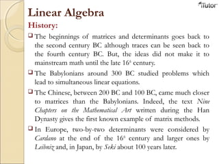
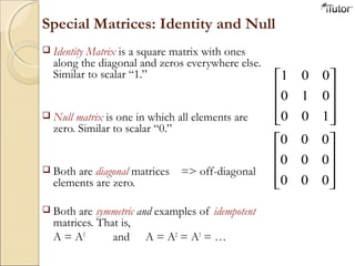
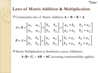
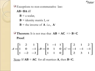
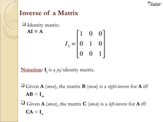
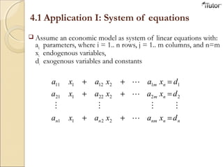
The document provides an overview of linear algebra and matrix theory. It discusses the history and development of matrices, defines key matrix concepts like dimensions and operations, and covers foundational topics like matrix addition, multiplication, inverses, and solving systems of linear equations. The document is intended as an introduction to linear algebra and matrices for students.

![Examples:
[ ]δβα=
−
= b
d
b
A ;
1
1
Dimensions of a matrix:
Numbers of rows by numbers of columns. The Matrix A is
a 2x2 matrix, b is a 1x3 matrix.
A matrix with only one column or only one row is called a
vector.
If a matrix has an equal numbers of rows and columns, it is
called a square matrix. Matrix A, above, is a square matrix.
Usual Notation: Upper case letters => matrices
Lower case => vectors](https://image.slidesharecdn.com/matrix-130924233933-phpapp01/85/Linear-Algebra-and-Matrix-4-320.jpg)
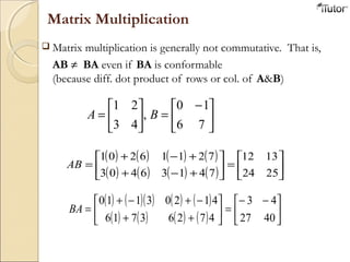
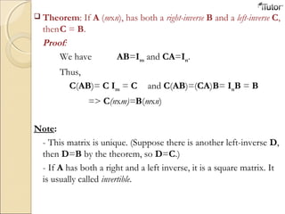
![Matrix multiplication
Multiplication of matrices requires a conformability condition
The conformability condition for multiplication is that the
column dimensions of the lead matrix A must be equal to the
row dimension of the lag matrix B.
If A is an (m x n) and B an (n x p) matrix (A has the same
number of columns a B has rows), then we define the product
of AB. AB is (m x p) matrix with its ij-th element is
What are the dimensions of the vector, matrix, and result?
[ ] [ ]131211
232221
131211
1211 cccc
bb
bbb
aaaB ==
=
[ ]231213112212121121121111 babababababa +++=
Dimensions: a(1 x 2), B(2 x 3) => c (1 x 3)
jk
n
j ijba∑ =1](https://image.slidesharecdn.com/matrix-130924233933-phpapp01/85/Linear-Algebra-and-Matrix-5-320.jpg)
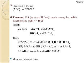
![Transpose Matrix
−
=′=>
−
=
49
08
13
401
983
AA:Example
The transpose of a matrix A is another matrix AT
(also written A
′) created by any one of the following equivalent actions:
- Write the rows (columns) of A as the columns (rows) of AT
- Reflect A by its main diagonal to obtain AT
Formally, the (i, j) element of AT
is the (j, i) element of A:
[AT
]ij
= [A]ji
If A is a m × n matrix => AT
is a n × m matrix.
(A')' = A
Conformability changes unless the matrix is square.](https://image.slidesharecdn.com/matrix-130924233933-phpapp01/85/Linear-Algebra-and-Matrix-6-320.jpg)
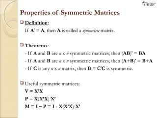
![ Examples:
[ ]
[ ]
//
2
/
1
'
2
'
1
'
2
'
1
02
2412
105
2410
125
=−
=
=
=
vv
v
v
v
v
[ ] [ ]
[ ]
023
54
162216
23
5
4
;
8
1
;
7
2
321
3
21
321
=−−
==
−=
−
=
=
=
vvv
v
vv
vvv](https://image.slidesharecdn.com/matrix-130924233933-phpapp01/85/Linear-Algebra-and-Matrix-24-320.jpg)