Download to read offline

![Optimality Conditions
LASSO problem
minimise 1
2 Ax − y 2
f
+ λ x 1
g
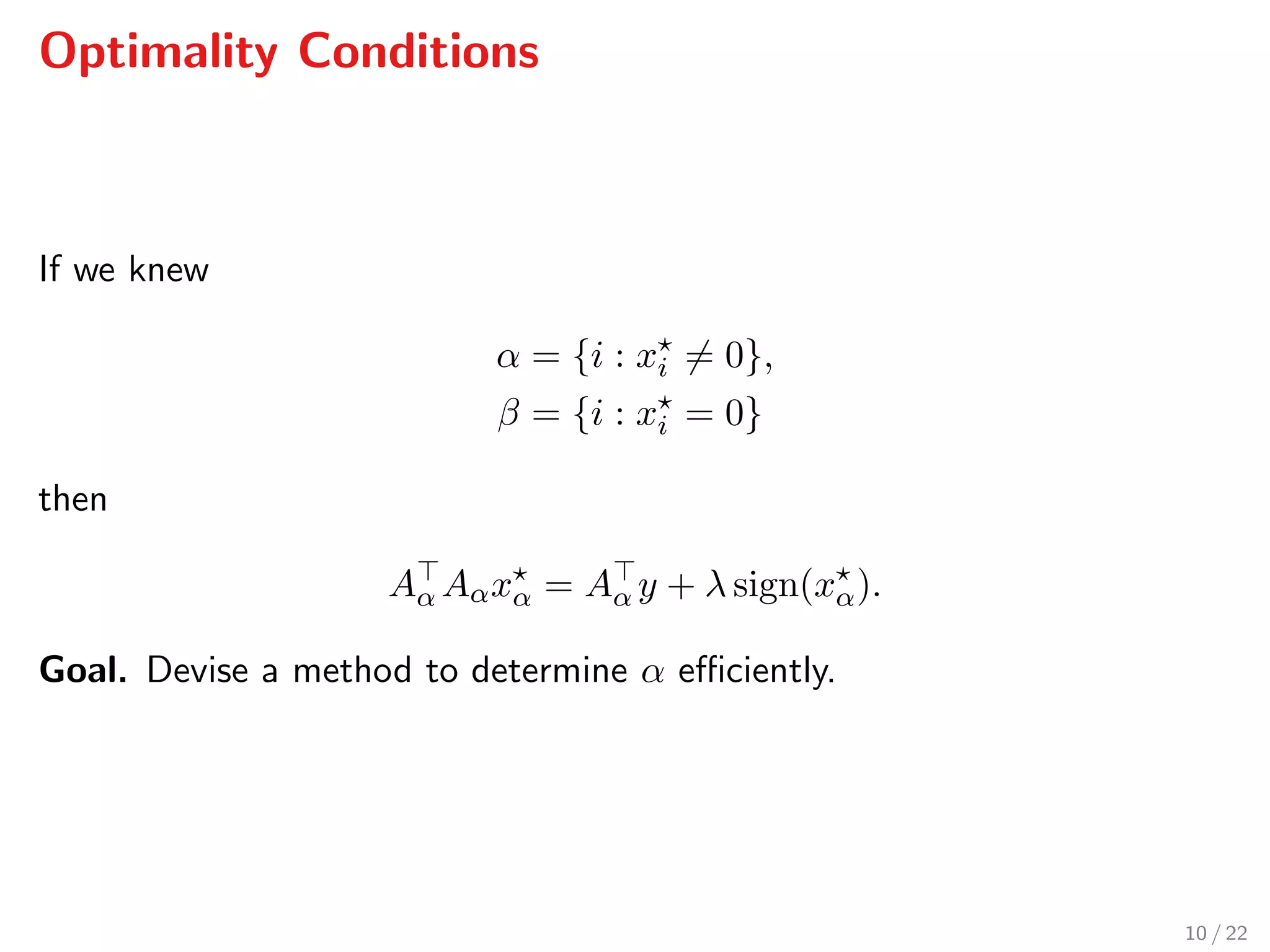
Optimality conditions:
− f(x ) ∈ ∂g(x ),
with f(x) = A (Ax − y) and ∂g(x)i = λ sign(xi) for xi = 0,
∂g(x)i = [−λ, λ] for xi = 0, so
− if(x ) = λ sign(xi ), for xi = 0,
| jf(x )| ≤ λ, for xj = 0
9 / 22](https://image.slidesharecdn.com/sopasakis-eusipco-2016-160905121324/75/Accelerated-reconstruction-of-a-compressively-sampled-data-stream-12-2048.jpg)


![Simulations
For a 10%-sparse stream
Window size ×10 4
0.5 1 1.5 2
Averageruntime[s]
10 -1
10 0
10 1
FBN
FISTA
ADMM
L1LS
19 / 22](https://image.slidesharecdn.com/sopasakis-eusipco-2016-160905121324/75/Accelerated-reconstruction-of-a-compressively-sampled-data-stream-23-2048.jpg)
![Simulations
For n = 5000 and different sparsities
Sparsity [%]
0 5 10 15
Averageruntime[s]
10 -1
10 0
FBN
FISTA
ADMM
L1LS
20 / 22](https://image.slidesharecdn.com/sopasakis-eusipco-2016-160905121324/75/Accelerated-reconstruction-of-a-compressively-sampled-data-stream-24-2048.jpg)


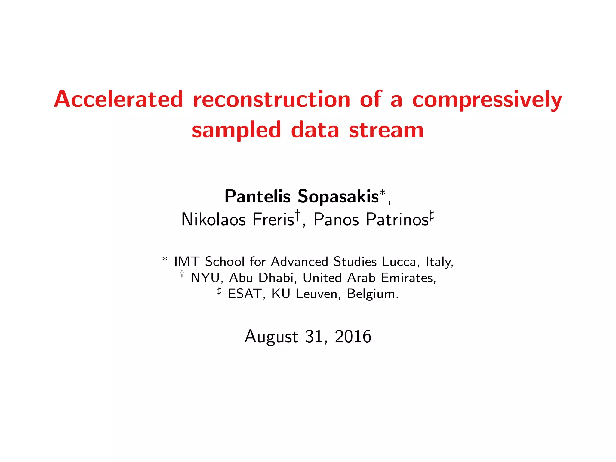
The document presents a novel methodology for accelerated reconstruction of compressively sampled data, achieving a speed that is an order of magnitude faster than existing recursive compressed sensing methods. It details the problem of retrieving sparse signals from noisy measurements, discusses the required properties of sampling matrices, and outlines the algorithmic approach using forward-backward Newton optimality conditions. Numerical simulations demonstrate the proposed method's significant performance advantages over traditional techniques like ISTA and FISTA.