The document describes a signal processing approach to fair surface design using Taubin smoothing. It discusses the theory behind Laplacian and Taubin smoothing algorithms and how they can be used to eliminate high frequencies from mesh surfaces. The implementation section details how the Laplacian operator, smoothing operator, and various constraints are implemented. Results show that Taubin smoothing can effectively reduce noise in models while preserving overall shape and that it can smooth voxelized CT scan data to produce fine visualizations of bone structures.
![5
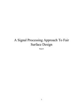
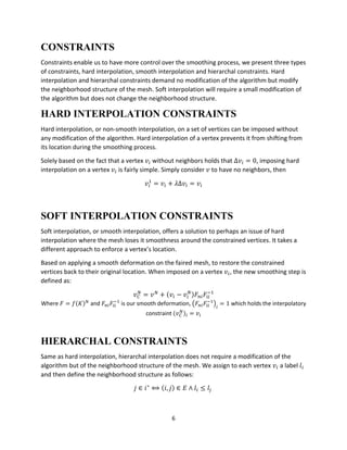
EIGENVALUES AND FREQUENCIES
The eigenvalues of the Laplacian operator 𝐾 are the frequencies of the mesh. In this part, we’ll
show how the Taubin Smoothing algorithm helps eliminating the high frequencies and
preserving the lower ones.
We first look at our weight function 𝑊 which, as mentioned above, must hold that all its
elements are non-negative and each row sums up to 1. Such matrices are called stochastic
matrices, and since 𝑊 is symmetric, the eigenvalues of 𝑊, denoted as 𝑘𝑖
𝑊
, are real and hold
|𝑘𝑖
𝑊
| ≤ 1
And by 𝐾’s construction, the eigenvalues of 𝐾 hold
0 ≤ 𝑘1
𝐾
≤ 𝑘2
𝐾
≤ ⋯ ≤ 𝑘 𝑛
𝐾
≤ 2
Real, bonded below by 0, and above by 2
In the case where 𝑊 is not symmetric, its eigenvalues might not be real, and the behavior of
the fairing algorithm will depend on their distribution in the complex plane. Although if the
eigenvalues are very close to the real line, we can ignore their imaginary parts and the result of
the algorithm should be essentially the same as the symmetric case above.
By 𝑓(𝐾)’s construction
𝑓(𝑘𝑖) = (1 − 𝜆𝑘𝑖)(1 − 𝜇𝑘𝑖)
The eigenvalues of 𝑓(𝐾)
PASS-BAND REGION
𝑓(𝑘) is a square function, since 𝑓(0) = 1 and 𝜆 + 𝜇 < 0, there is a positive 𝑘 𝑝𝑏 called the pass-
band frequency which holds 𝑓(𝑘 𝑝𝑏) = 1. And then
∀𝑘 ∈ [0, 𝑘 𝑝𝑏], 𝑓(𝑘) 𝑁
≈ 1
Pass-band region is preserved and
∀𝑘 ∈ (𝑘 𝑝𝑏, 2], 𝑓(𝑘) 𝑁
≈ 0 for large enough 𝑁
By demanding 𝑓(𝑘) = 1 we find that
𝑘 𝑝𝑏 =
1
𝜇
+
1
𝜆
To minimize the number of iterations, 𝑁, the smoothing strength factor 𝜆 must be as large as
possible while keeping ∀𝑘 ∈ (𝑘 𝑝𝑏, 2], |𝑓(𝑘)| < 1.](https://image.slidesharecdn.com/6ce5ffee-fb73-46dc-8fd4-ff5f926791e3-161213143445/85/A-Signal-Processing-Approach-To-Fair-Surface-Design-5-320.jpg)
![7
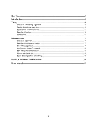
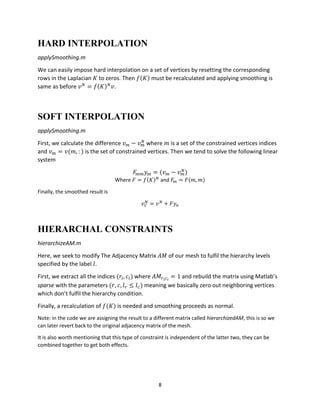
IMPLEMENTATION
LAPLACIAN OPERATOR
getEdgeLengthWeights.m, getNeighorWeights.m, getK.m
We start by defining our Laplacian operator
𝐾 = 𝐼 − 𝑊
Where 𝑊 can be chosen to be either the inverse length of edges (𝑤𝑖𝑗) =
‖𝑝 𝑖−𝑝 𝑗‖
−1
∑ ‖𝑝 𝑖−𝑝ℎ‖−1
ℎ∈𝑖∗
, or the
neighbor(uniform) weights (𝑤𝑖𝑗) =
1
|𝑖∗|
PASS-BAND REGION AND FACTORS
getLambdaMiu.m
The easiest way to achieve control over the smoothing process, is to choose a pass-band
frequency 𝑘 𝑝𝑏 first and deduct the values 𝜆 and 𝜇 from it. To do that we tend to solve the
following non-linear equation system
{
𝑘 𝑝𝑏 =
1
𝜆
+
1
𝜇
𝑓(1) = −𝑓(2)
The system was solved using Matlab’s fsolver with the initial guess 𝜆0 = 0.5 , 𝜇0 = −0.5.
For most meshes, a value of 𝑘 𝑝𝑏 in the region [0.01,0.1] produced best results.
SMOOTHING OPERATOR
getfK.m, applySmoothing.m
Finally, we can define our smoothing operator
𝑓(𝐾) = (𝐼 − 𝜆𝐾)(𝐼 − 𝜇𝐾)
We’ve also added the option to get the Laplacian smoothing operator 𝑓(𝐾) = (𝐼 − 𝜆𝐾)
Applying the operator is simple, the result of the smoothing after 𝑁 iterations is as mentioned
before 𝑣 𝑁
= 𝑓(𝐾) 𝑁
𝑣](https://image.slidesharecdn.com/6ce5ffee-fb73-46dc-8fd4-ff5f926791e3-161213143445/85/A-Signal-Processing-Approach-To-Fair-Surface-Design-7-320.jpg)


![Av 738- Adaptive Filtering - Wiener Filters[wk 3]](https://cdn.slidesharecdn.com/ss_thumbnails/av-738-aft-spr18-lecture03-optimumfilters-weinerwk3-180215235757-thumbnail.jpg?width=640&height=640&fit=bounds)


![[Review] contact model fusion](https://cdn.slidesharecdn.com/ss_thumbnails/reviewcontactmodelfusion-200217071839-thumbnail.jpg?width=640&height=640&fit=bounds)


