Download as PDF, PPTX
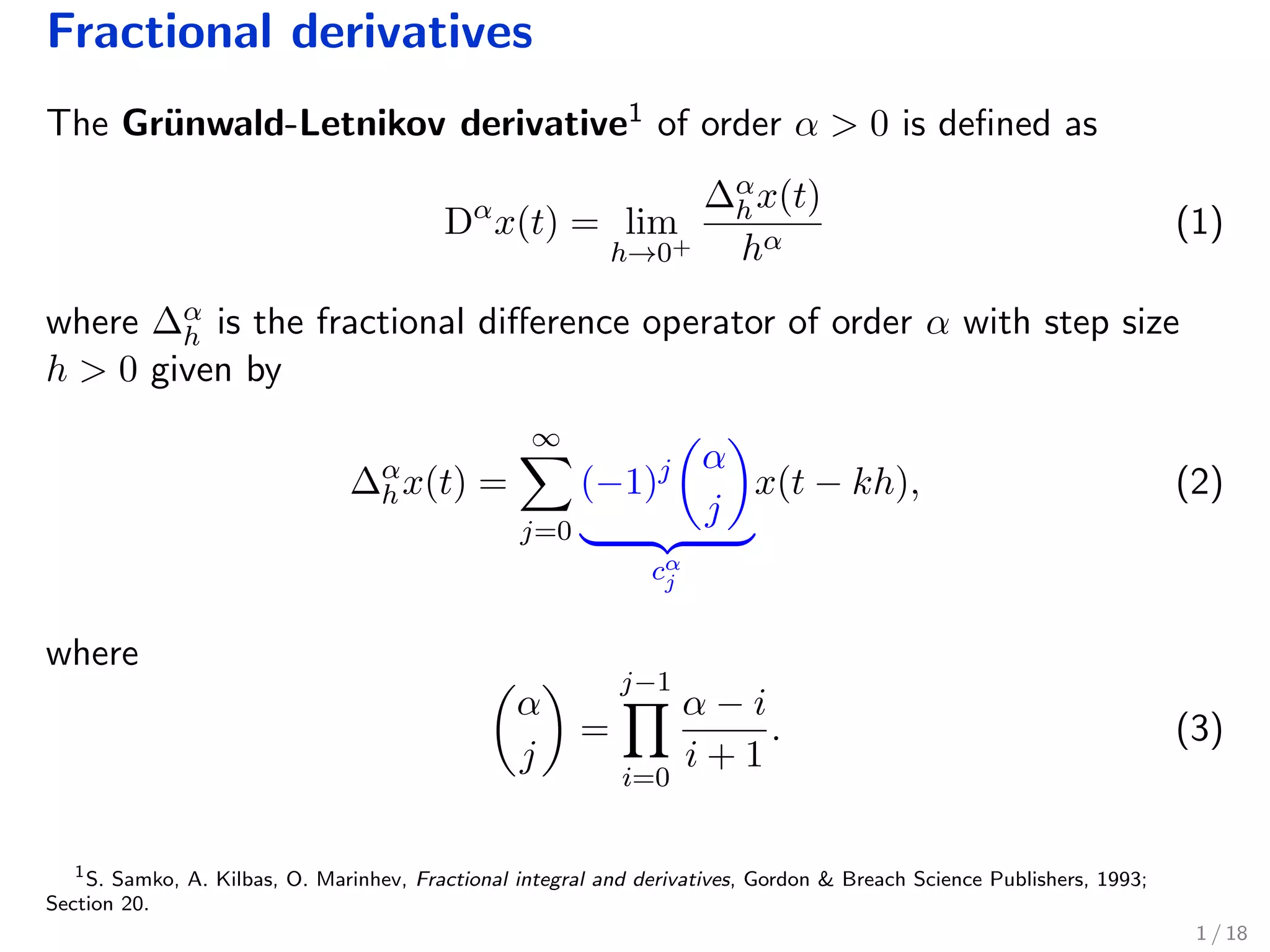
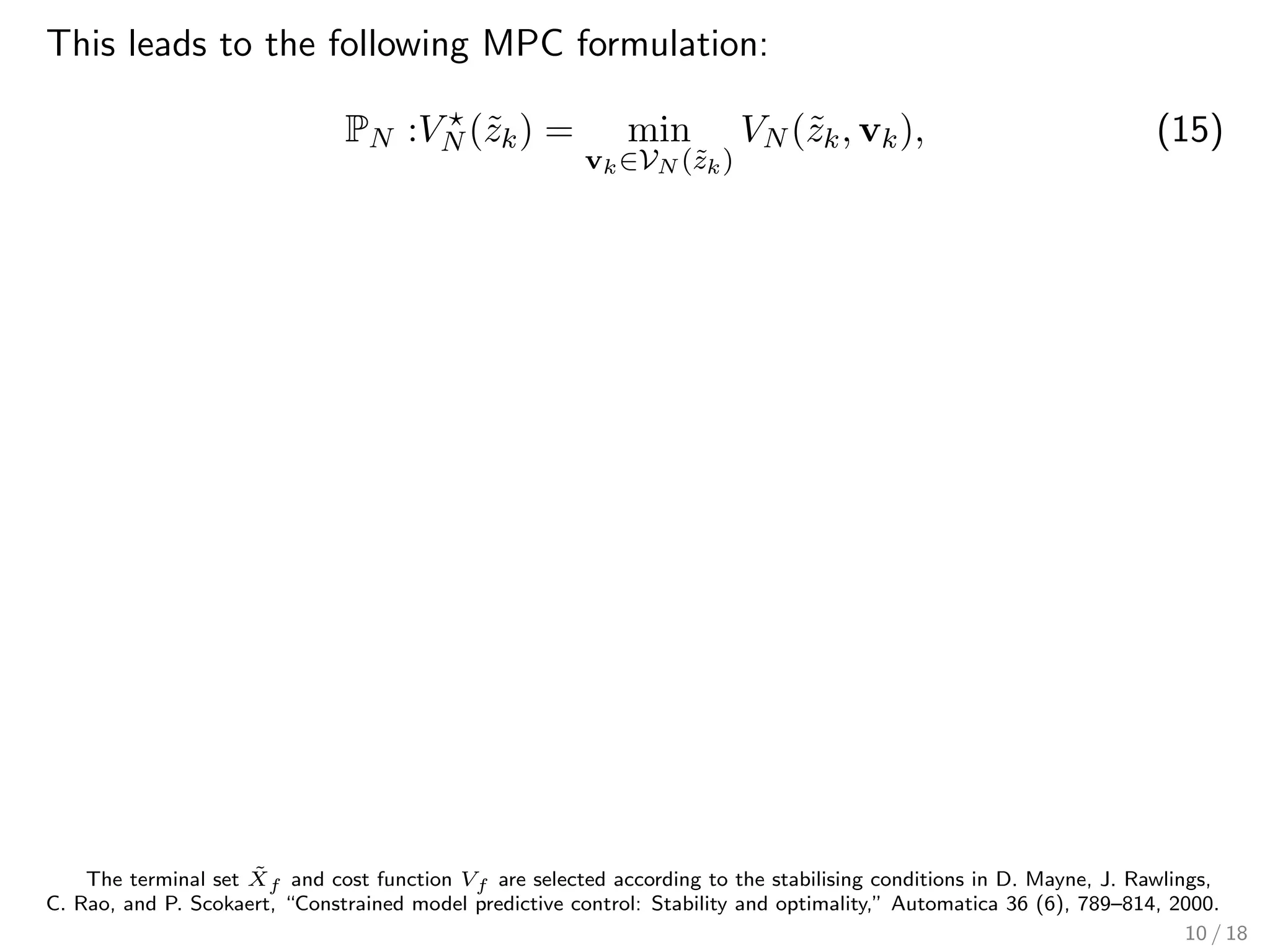
![Fractional systems
Fractional-order systems
l
i=1
AiDαi
x(t) = Bu(t) (4)
Euler-type discretisation [Replace Dαi h−αi ∆αi
h ]
l
i=1
¯Ai∆αi
h xk+1 = Buk (5)
Notice that ∆αi
h is an infinite-dimensional operator!
3 / 18](https://image.slidesharecdn.com/medsopasakis-150618142506-lva1-app6892/75/Robust-model-predictive-control-for-discrete-time-fractional-order-systems-5-2048.jpg)
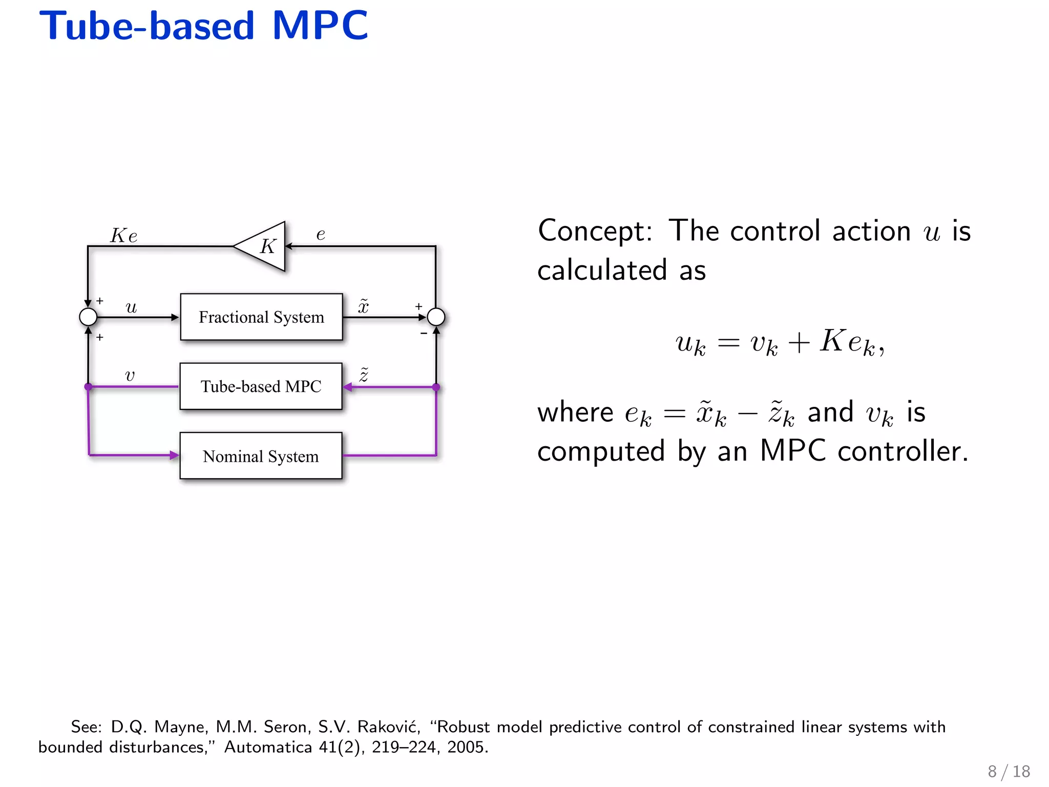
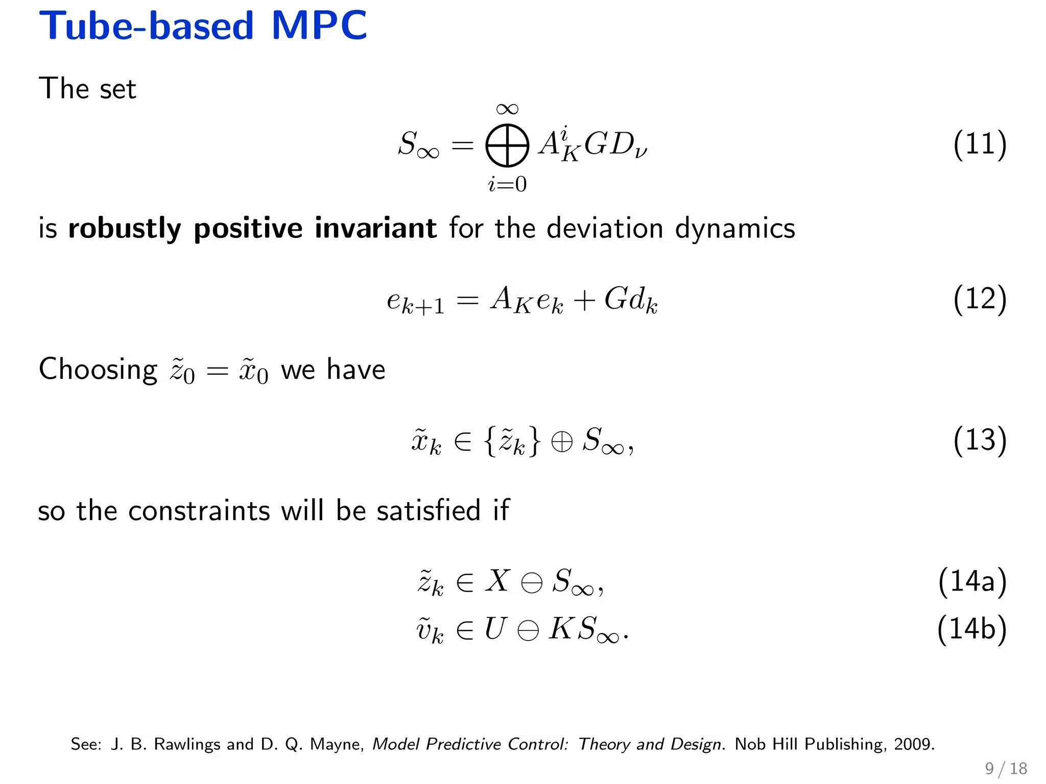
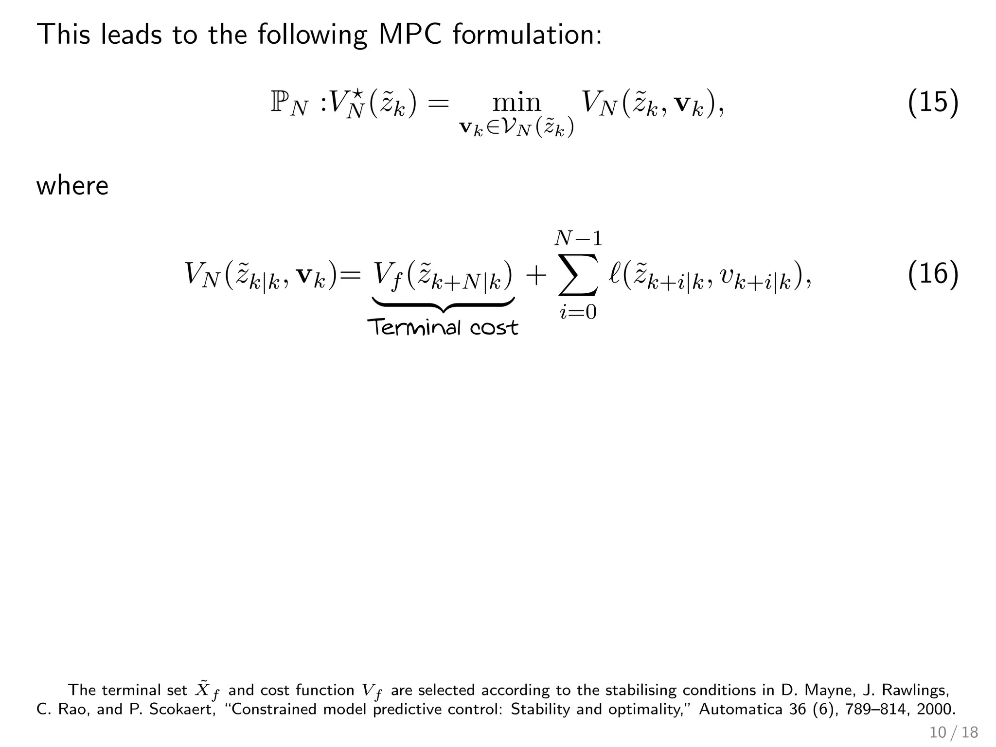
![This leads to the following MPC formulation:
PN :VN (˜zk) = min
vk∈VN (˜zk)
VN (˜zk, vk), (15)
where
VN (˜zk|k, vk)= Vf (˜zk+N|k)
Terminal cost
+
N−1
i=0
(˜zk+i|k, vk+i|k), (16)
and for some S ⊇ S∞
VN (˜zk)=
v
˜zk+i+1|k=A˜zk+i|k+Bvk+i|k, ∀i∈N[0,N−1]
˜zk|k = ˜zk
˜zk+i|k ∈ ˜X S, ∀i∈N[1,N]
vk+i|k ∈ U KS, ∀i∈N[0,N−1]
˜zk+N|k ∈ ˜Xf Terminal constraints
(17)
The terminal set ˜Xf and cost function Vf are selected according to the stabilising conditions in D. Mayne, J. Rawlings,
C. Rao, and P. Scokaert, “Constrained model predictive control: Stability and optimality,” Automatica 36 (6), 789–814, 2000.
10 / 18](https://image.slidesharecdn.com/medsopasakis-150618142506-lva1-app6892/75/Robust-model-predictive-control-for-discrete-time-fractional-order-systems-15-2048.jpg)

![Is the controlled system asymptotically stable?
We have shown that the following condition entails asymptotic stability
properties for the controlled system:
j∈N
Aj
KG
i∈N[1,l]
− ˆA−1
0
¯AiΨν(αi)Bn
⊆ B¯n
,
for some > 0.](https://image.slidesharecdn.com/medsopasakis-150618142506-lva1-app6892/75/Robust-model-predictive-control-for-discrete-time-fractional-order-systems-29-2048.jpg)

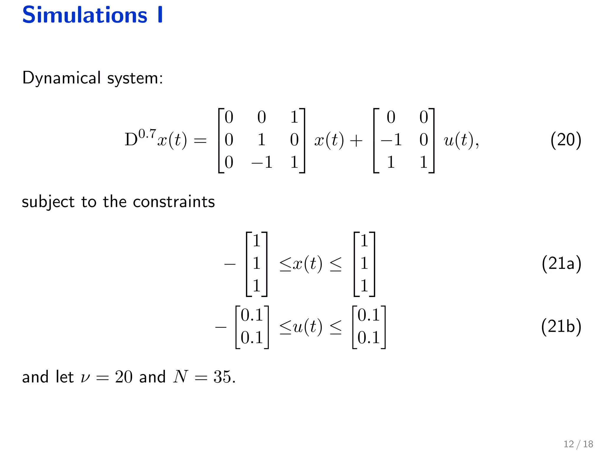
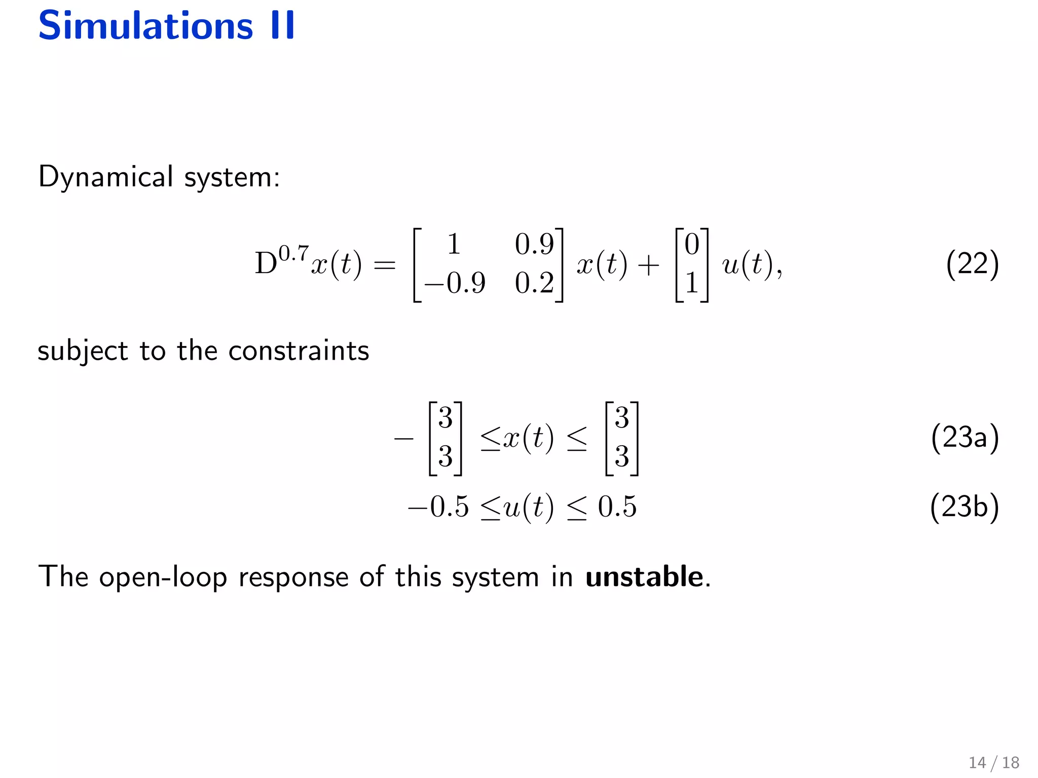
The document discusses robust model predictive control (MPC) for fractional-order discrete-time systems and introduces finite-dimensional approximations using fractional derivatives. It highlights the relevance of fractional systems in various applications, including pharmacokinetics and electromagnetic theory, and presents an MPC formulation that ensures constraints are met within a robustly positive invariant set. Simulations illustrate the approach's effectiveness, while also addressing ongoing questions regarding stability and application to controlled drug administration.


![Circuit Network Analysis - [Chapter4] Laplace Transform](https://cdn.slidesharecdn.com/ss_thumbnails/ch4-150613063858-lva1-app6891-thumbnail.jpg?width=640&height=640&fit=bounds)