Download as PDF, PPTX


![Demand forecasting
Common approaches:
1. Neglect the error: ( 0, 1, . . . , N ) (0, 0, . . . , 0)
2. Error bounds: ( 0, 1, . . . , N ) ∈ E, e.g., j ∈ [ min
j , max
j ]
25 / 89](https://image.slidesharecdn.com/ascona-sopasakis-160824134758/85/Smart-Systems-for-Urban-Water-Demand-Management-29-320.jpg)
![Demand forecasting
Common approaches:
1. Neglect the error: ( 0, 1, . . . , N ) (0, 0, . . . , 0)
2. Error bounds: ( 0, 1, . . . , N ) ∈ E, e.g., j ∈ [ min
j , max
j ]
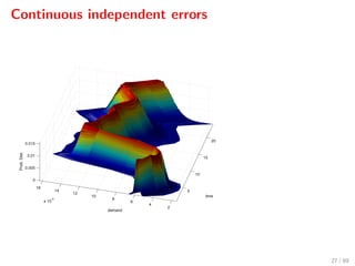
3. Independent normal distributions: j ∼ N(mj, σ2
j )
25 / 89](https://image.slidesharecdn.com/ascona-sopasakis-160824134758/85/Smart-Systems-for-Urban-Water-Demand-Management-30-320.jpg)
![Demand forecasting
Common approaches:
1. Neglect the error: ( 0, 1, . . . , N ) (0, 0, . . . , 0)
2. Error bounds: ( 0, 1, . . . , N ) ∈ E, e.g., j ∈ [ min
j , max
j ]
3. Independent normal distributions: j ∼ N(mj, σ2
j )
4. ( 0, 1, . . . , N ) is random and admits finitely many values
25 / 89](https://image.slidesharecdn.com/ascona-sopasakis-160824134758/85/Smart-Systems-for-Urban-Water-Demand-Management-31-320.jpg)
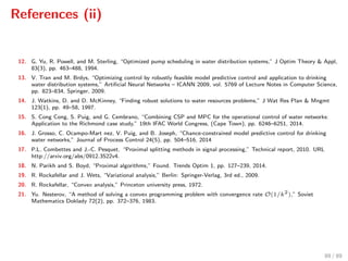
![Error bounds
0 20 40 60 80 100 120 140 160 180 200
0
0.01
0.02
0.03
0.04
0.05
0.06
0.07
Time [h]
WaterDemandFlow[m
3
/h]
Forecasting of Water Demand
FuturePast
26 / 89](https://image.slidesharecdn.com/ascona-sopasakis-160824134758/85/Smart-Systems-for-Urban-Water-Demand-Management-32-320.jpg)
![Predicted scenarios
Time [hr]
4370 4380 4390 4400 4410 4420 4430
Waterdemand[m
3
/s]
0.01
0.015
0.02
0.025
0.03
0.035
0.04
0.045
0.05
28 / 89](https://image.slidesharecdn.com/ascona-sopasakis-160824134758/85/Smart-Systems-for-Urban-Water-Demand-Management-34-320.jpg)
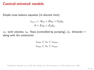
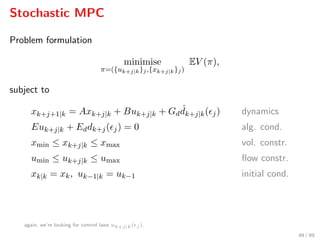
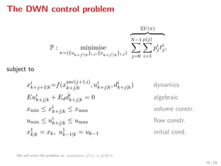
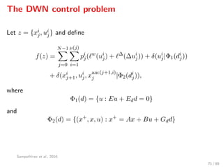
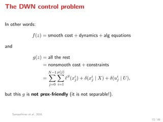
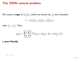
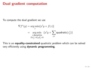
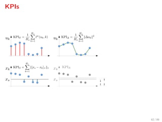
![Control objectives
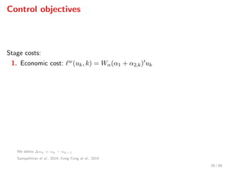
Stage costs:
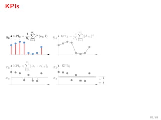
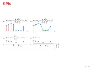
1. Economic cost: w(uk, k) = Wα(α1 + α2,k) uk
2. Smooth operation cost: ∆(∆uk) = ∆ukWu∆uk
3. Safe operation cost: S(xk) = Wx [xs − xk]+
We define ∆uk = uk − uk−1
Sampathirao et al., 2014; Cong Cong et al., 2014
29 / 89](https://image.slidesharecdn.com/ascona-sopasakis-160824134758/85/Smart-Systems-for-Urban-Water-Demand-Management-37-320.jpg)
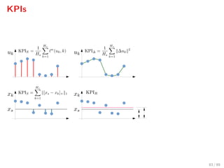
![Control objectives
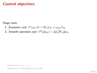
Stage costs:
1. Economic cost: w(uk, k) = Wα(α1 + α2,k) uk
2. Smooth operation cost: ∆(∆uk) = ∆ukWu∆uk
3. Safe operation cost: S(xk) = Wx [xs − xk]+
4. Total cost: = w + ∆ + S.
We define ∆uk = uk − uk−1
Sampathirao et al., 2014; Cong Cong et al., 2014
29 / 89](https://image.slidesharecdn.com/ascona-sopasakis-160824134758/85/Smart-Systems-for-Urban-Water-Demand-Management-38-320.jpg)

![Closed-loop simulations
20 40 60 80 100 120 140 160
Controlaction[%]
0
0.2
0.4
0.6
0.8
Time [hr]
20 40 60 80 100 120 140 160
WaterCost[e.u.]
60
70
80
90
86 / 89](https://image.slidesharecdn.com/ascona-sopasakis-160824134758/85/Smart-Systems-for-Urban-Water-Demand-Management-101-320.jpg)
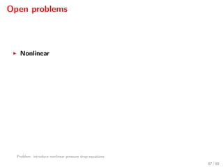
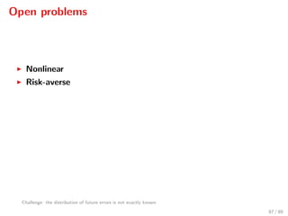
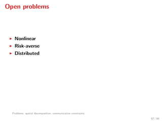


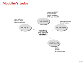
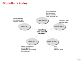
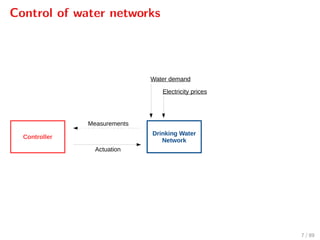
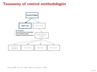
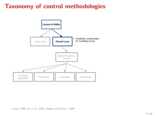
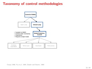
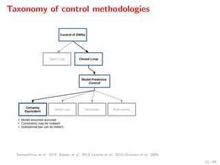
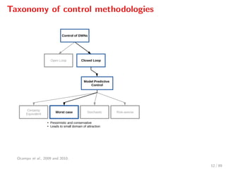
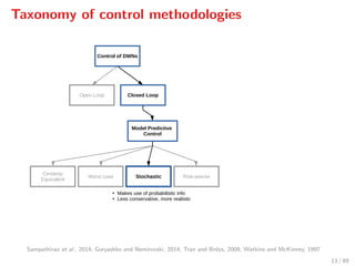
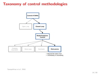
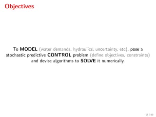
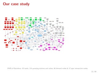
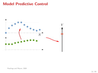
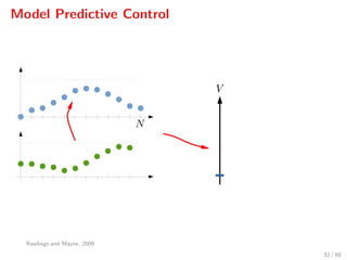
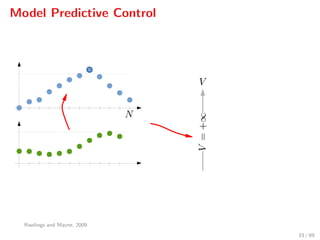
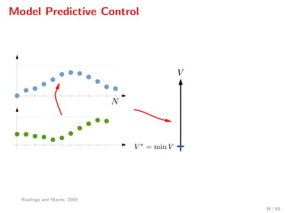
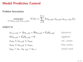
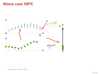
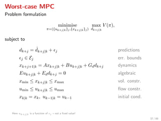
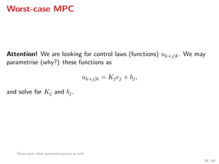
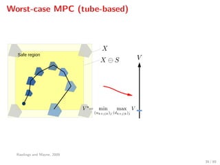
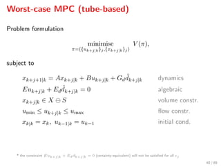
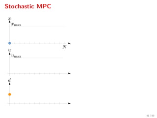
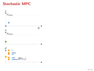
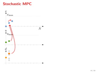
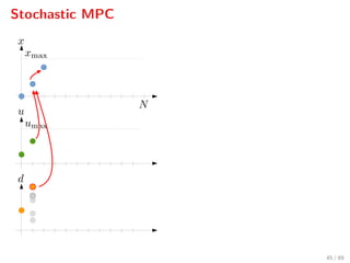
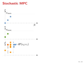
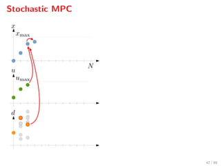
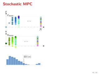
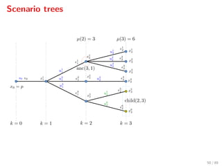
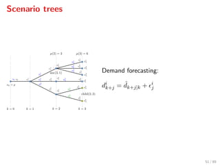
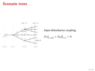
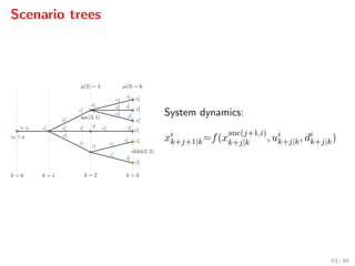
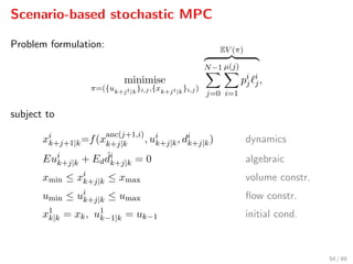
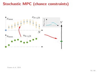
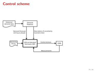
The document discusses advanced methodologies for modeling and controlling urban water networks, focusing on demand management and decision-making under uncertainty. It covers model predictive control (MPC) concepts, various control strategies including stochastic and worst-case MPC, and the importance of forecasting demand while considering constraints and objectives such as economic and safe operation costs. The case study illustrates the application of these methodologies to the water distribution network of Barcelona.


