Download as PDF, PPTX
![Forward-Backward Splitting
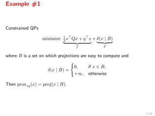
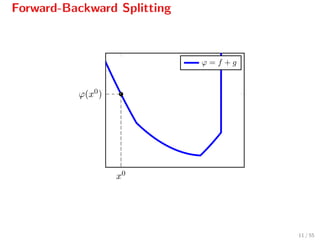
Problem structure
minimize ϕ(x) = f(x) + g(x)
where
1. f, g : Rn → ¯R are proper, closed, convex
2. f has L-Lipschitz gradient
3. g is prox-friendly, i.e., its proximal operator
proxγg(v) := arg min
z
g(z) + 1
2 v − z 2
is easily computable[1]
.
[1]
Parikh & Boyd 2014; Combettes & Pesquette, 2010.
4 / 55](https://image.slidesharecdn.com/rcs-160412145939/85/Recursive-Compressed-Sensing-6-320.jpg)
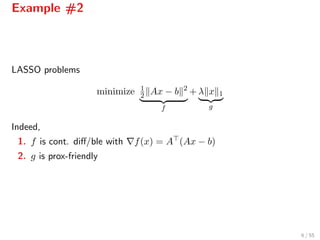
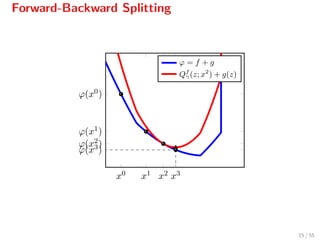
![Forward-Backward Splitting
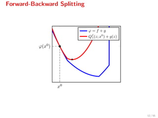
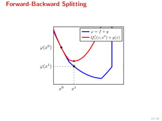
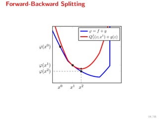
The iteration
xk+1
= proxγg(xk
− γ f(xk
)),
can be written as[2]
xk+1
= arg min
z
f(xk
) + f(xk
), z − xk
+ 1
2γ z − xk 2
Qf
γ(z,xk)
+g(z) ,
where Qf
γ(z, xk) serves as a quadratic model for f[3]
.
[2]
Beck and Teboulle, 2010.
[3]
Qf
γ (·, xk
) is the linearization of f at xk
plus a quadratic term; moreover, Qf
γ (z, xk
) ≥ f(x) and Qf
γ (z, z) = f(z).
9 / 55](https://image.slidesharecdn.com/rcs-160412145939/85/Recursive-Compressed-Sensing-11-320.jpg)

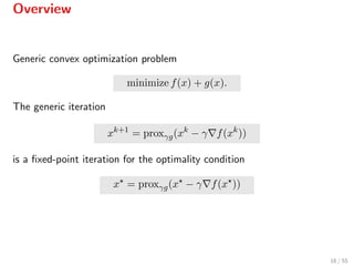
![Overview
It generalizes several other methods
xk+1
=
xk − γ f(xk) gradient method, g = 0
ΠC(xk − γ f(xk)) gradient projection, g = δ(· | C)
proxγg(xk) proximal point algorithm, f = 0
There are several flavors of proximal gradient algorithms[4]
.
[4]
Nesterov’s accelerated method, FISTA (Beck & Teboulle), etc.
17 / 55](https://image.slidesharecdn.com/rcs-160412145939/85/Recursive-Compressed-Sensing-19-320.jpg)
![Shortcomings
FBS are first-order methods, therefore, they can be slow!
Overhaul. Use a better quadratic model for f[5]
:
Qf
γ,B(z, xk
) = f(xk
) + f(xk
), z − xk
+ 1
2γ z − xk 2
Bk ,
where Bk is (an approximation of) 2f(x).
Drawback. No closed form solution of the inner problem.
[5]
As in Becker & Fadili 2012; Lee et al. 2012; Tran-Dinh et al. 2013.
18 / 55](https://image.slidesharecdn.com/rcs-160412145939/85/Recursive-Compressed-Sensing-20-320.jpg)
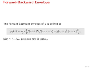
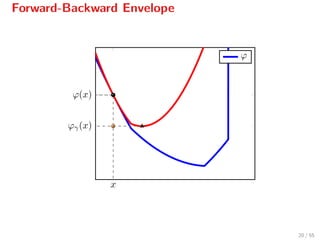
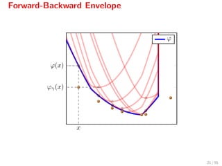
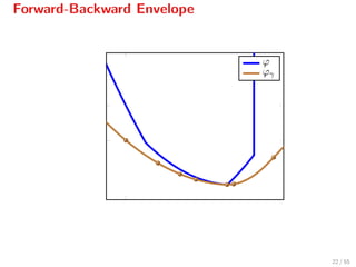
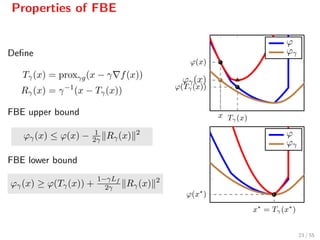
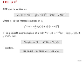
![Properties of FBE
Ergo: Minimizing ϕ is equivalent to minimizing its FBE ϕγ.
inf ϕ = inf ϕγ
arg min ϕ = arg min ϕγ
However, ϕγ is continuously diff/able[6]
whenever f ∈ C2.
[6]
More about the FBE: P. Patrinos, L. Stella and A. Bemporad, 2014.
24 / 55](https://image.slidesharecdn.com/rcs-160412145939/85/Recursive-Compressed-Sensing-27-320.jpg)
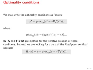
![Optimality conditions
LASSO problem
minimize 1
2 Ax − b 2
f
+ λ x 1
g
.
Optimality conditions
− f(x ) ∈ ∂g(x ).
where f(x) = A (Ax − b) and ∂g(x)i = λ sign(xi) for xi = 0 and
∂g(x)i = [−λ, λ] otherwise, so
− if(x ) = λ sign(xi ), if xi = 0,
| if(x )| ≤ λ, otherwise
28 / 55](https://image.slidesharecdn.com/rcs-160412145939/85/Recursive-Compressed-Sensing-32-320.jpg)

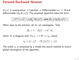
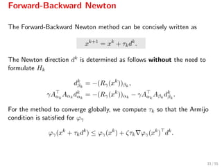
![B-subdifferential
For a function F : Rn → Rn which is almost everywhere differentiable, we
define its B-subdifferential to be[7]
∂BF(x) := B ∈ Rn×n ∃{xn}n : xn → x,
Rγ(xn) exists and Rγ(xn) → B
.
[7]
See Facchinei & Pang, 2004
31 / 55](https://image.slidesharecdn.com/rcs-160412145939/85/Recursive-Compressed-Sensing-35-320.jpg)
![Speeding up FBN by Continuation
1. In applications of LASSO we have x 0 ≤ m n[8]
[8]
The zero-norm of x, x 0, is the number of its nonzeroes.
35 / 55](https://image.slidesharecdn.com/rcs-160412145939/85/Recursive-Compressed-Sensing-39-320.jpg)
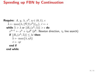
![Speeding up FBN by Continuation
1. In applications of LASSO we have x 0 ≤ m n[8]
2. If λ ≥ λ0 := f(x0) ∞, then supp(x) = ∅
[8]
The zero-norm of x, x 0, is the number of its nonzeroes.
35 / 55](https://image.slidesharecdn.com/rcs-160412145939/85/Recursive-Compressed-Sensing-40-320.jpg)
![Speeding up FBN by Continuation
1. In applications of LASSO we have x 0 ≤ m n[8]
2. If λ ≥ λ0 := f(x0) ∞, then supp(x) = ∅
3. We relax the optimization problem solving
P(¯λ) : minimize 1
2 Ax − y 2
+ ¯λ x 1
[8]
The zero-norm of x, x 0, is the number of its nonzeroes.
35 / 55](https://image.slidesharecdn.com/rcs-160412145939/85/Recursive-Compressed-Sensing-41-320.jpg)
![Speeding up FBN by Continuation
1. In applications of LASSO we have x 0 ≤ m n[8]
2. If λ ≥ λ0 := f(x0) ∞, then supp(x) = ∅
3. We relax the optimization problem solving
P(¯λ) : minimize 1
2 Ax − y 2
+ ¯λ x 1
4. Once we have approximately solved P(¯λ) we update ¯λ as
¯λ ← max{η¯λ, λ},
until eventually ¯λ = λ.
[8]
The zero-norm of x, x 0, is the number of its nonzeroes.
35 / 55](https://image.slidesharecdn.com/rcs-160412145939/85/Recursive-Compressed-Sensing-42-320.jpg)
![Speeding up FBN by Continuation
1. In applications of LASSO we have x 0 ≤ m n[8]
2. If λ ≥ λ0 := f(x0) ∞, then supp(x) = ∅
3. We relax the optimization problem solving
P(¯λ) : minimize 1
2 Ax − y 2
+ ¯λ x 1
4. Once we have approximately solved P(¯λ) we update ¯λ as
¯λ ← max{η¯λ, λ},
until eventually ¯λ = λ.
5. This way we enforce that (i) |αk| increases smoothly, (ii) |αk| < m,
(iii) Aαk
Aαk
remains always positive definite.
[8]
The zero-norm of x, x 0, is the number of its nonzeroes.
35 / 55](https://image.slidesharecdn.com/rcs-160412145939/85/Recursive-Compressed-Sensing-43-320.jpg)
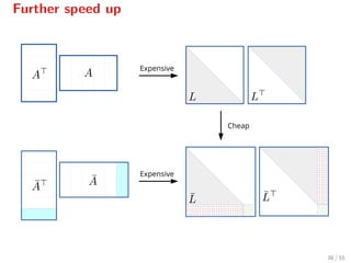
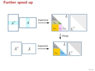
![Further speed up
When Aα is positive definite[9]
, we may compute a Cholesky factorization
of Aα0
Aα0 and then update the Cholesky factorization of Aαk+1
Aαk+1
using the factorization of Aαk
Aαk
.
[9]
In practice, always (when the continuation heuristic is used). Furthermore, α0 = ∅.
37 / 55](https://image.slidesharecdn.com/rcs-160412145939/85/Recursive-Compressed-Sensing-45-320.jpg)


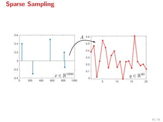
![Sparse Sampling
We require that A satisfies the restricted isometry property[10]
, that is
(1 − δs) x 2
≤ Ax 2
≤ (1 + δs) x 2
A typical choice is a random matrix A with entries drawn from N(0, 1
m )
with m = 4s.
[10]
This can be established using the Johnson-Lindenstrauss lemma.
43 / 55](https://image.slidesharecdn.com/rcs-160412145939/85/Recursive-Compressed-Sensing-52-320.jpg)
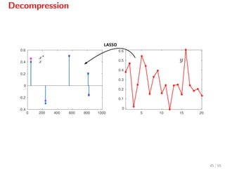
![Decompression
Assuming that
w ∼ N(0, σ2I),
the smallest element of |x| is not too small (> 8σ
√
2 ln n),
λ = 4σ
√
2 ln n,
the LASSO recovers the support of x[11]
, that is
x = arg min 1
2 Ax − y 2
+ λ x 1,
has the same support as the actual x.
[11]
Cand`es & Plan, 2009.
44 / 55](https://image.slidesharecdn.com/rcs-160412145939/85/Recursive-Compressed-Sensing-53-320.jpg)
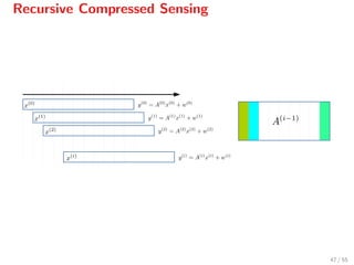
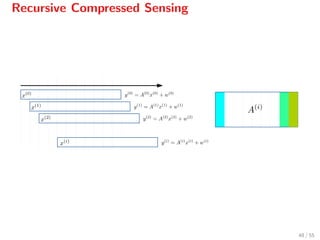
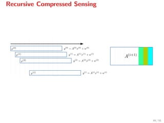
![Recursive Compressed Sensing
Define
x(i)
:= xi xi+1 · · · xi+n−1
Then x(i) produces the measured signal
y(i)
= A(i)
x(i)
+ w(i)
.
Sampling is performed with a constant matrix A[12]
and
A(0)
= A,
A(i+1)
= A(i)
P,
where P is a permutation matrix which shifts the columns of A leftwards.
[12]
For details see: N. Freris, O. ¨O¸cal and M. Vetterli, 2014.
46 / 55](https://image.slidesharecdn.com/rcs-160412145939/85/Recursive-Compressed-Sensing-55-320.jpg)
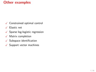
![Simulations
For a 10%-sparse stream
Window size ×10 4
0.5 1 1.5 2
Averageruntime[s]
10 -1
10 0
10 1
FBN
FISTA
ADMM
L1LS
52 / 55](https://image.slidesharecdn.com/rcs-160412145939/85/Recursive-Compressed-Sensing-62-320.jpg)
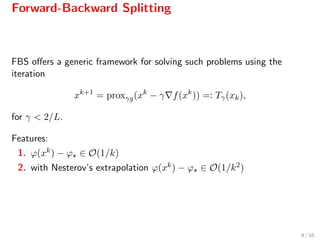
![Simulations
For n = 5000 varying the stream sparsity
Sparsity [%]
0 5 10 15
Averageruntime[s]
10 -1
10 0
FBN
FISTA
ADMM
L1LS
53 / 55](https://image.slidesharecdn.com/rcs-160412145939/85/Recursive-Compressed-Sensing-63-320.jpg)


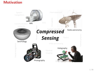
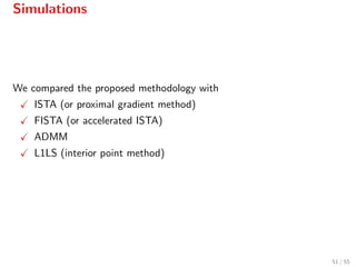
The document discusses a proposed method for recursive compressed sensing, demonstrating that it is significantly faster than existing methods. It covers various optimization techniques including forward-backward splitting and Newton methods, and their applications in solving sparse coding problems. Additionally, simulations and the implications of this method in fields like MRI, radio-astronomy, and medical imaging are highlighted.