The document discusses the natural gradient method for optimizing neural networks. It explains that the natural gradient finds the direction of steepest descent in function space rather than parameter space. The natural gradient is invariant to reparameterization. For most neural networks, natural gradient descent is equivalent to a second-order optimization method called the generalized Gauss-Newton method. The natural gradient takes into account the geometry of the parameter space defined by the Fisher information matrix.

1. 1 / 18
New Insights and Perspectives on the Natural
Gradient Method
Yoonho Lee
Department of Computer Science and Engineering
Pohang University of Science and Technology
March 13, 2018

2. 2 / 18
Motivation
In parameter space (µ, σ), each pair of distributions have the same
distance.

3. 3 / 18
Motivation
We often talk about the parameter space of a neural network,
instead of the functions that those parameters represent.

4. 4 / 18
Gradient Descent
The gradient descent update
∆θ = −α θL
is the solution to the following optimization problem:
arg min
∆θ
[ θL(θ) · ∆θ]
s.t. ∆θ ≤ δ.
We are optimizing a linear approximation of L within a trust region
defined by the Euclidean metric in parameter space.

5. 5 / 18
Natural Gradient
Consider a family of density functions F : θ → p(z) where θ ∈ Rn:
pθ(z) := F(θ)(z).
We naturally obtain a notion of closeness among different values of
θ:
d(θ1, θ2) := KL(pθ1 (z)||pθ2 (z)).

6. 6 / 18
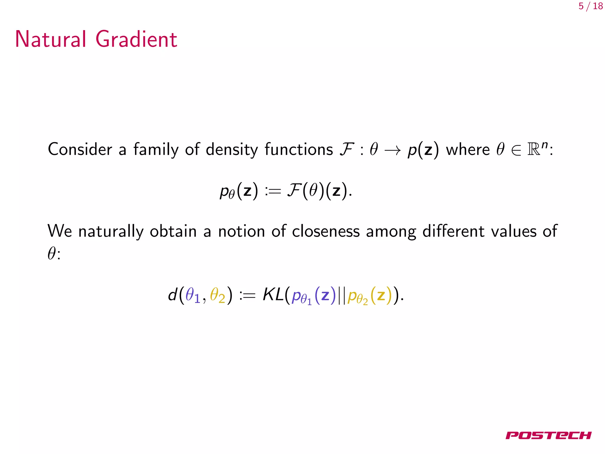
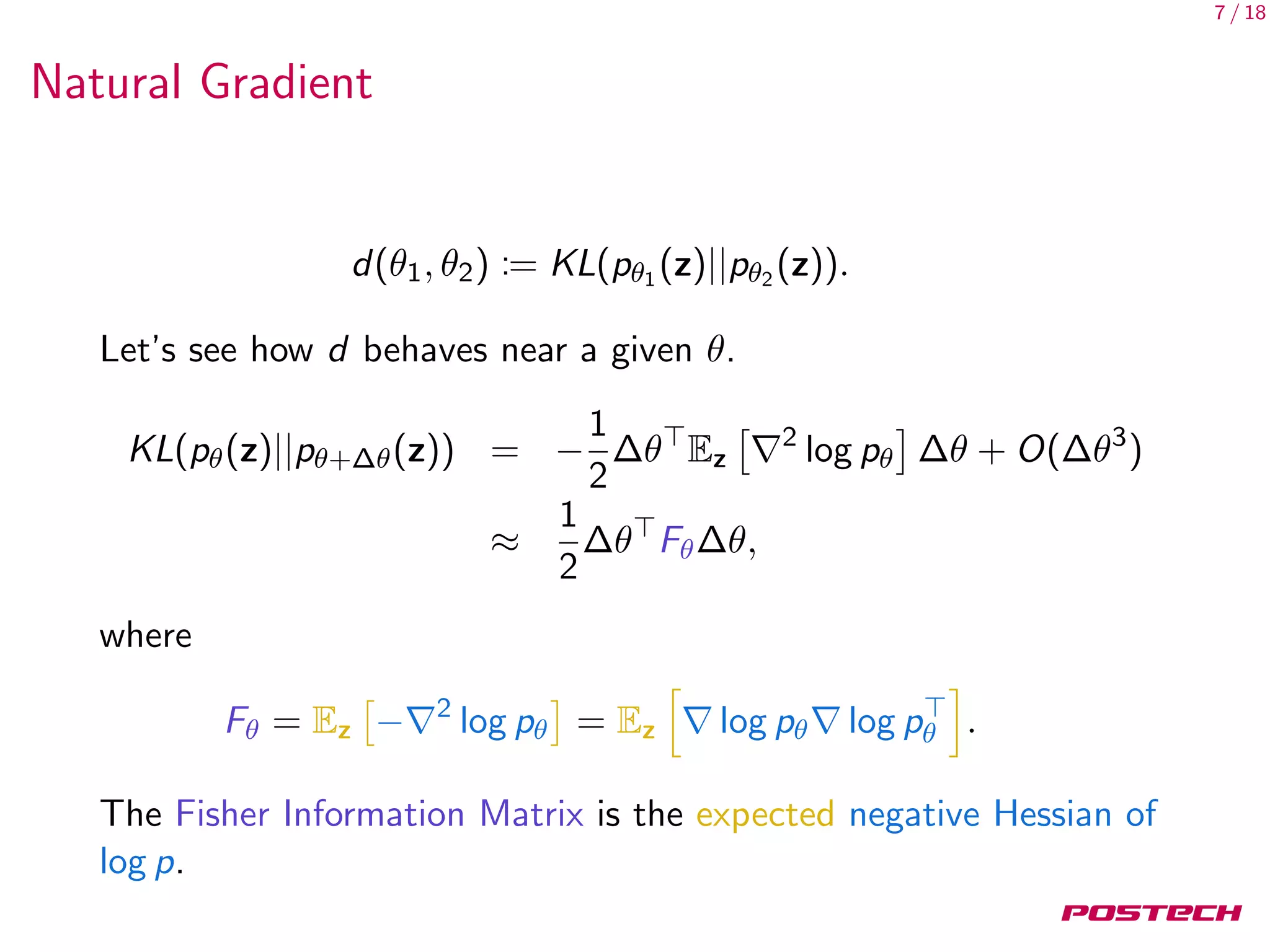
Natural Gradient
d(θ1, θ2) := KL(pθ1 (z)||pθ2 (z)).
Let’s see how d behaves near a given θ.
KL(pθ(z)||pθ+∆θ(z)) = Ez [log pθ] − Ez [log pθ]
−Ez [ log pθ] ∆θ + O(∆θ2
)
= O(∆θ2
),
so no useful information from first order approximation.

7. 7 / 18
Natural Gradient
d(θ1, θ2) := KL(pθ1 (z)||pθ2 (z)).
Let’s see how d behaves near a given θ.
KL(pθ(z)||pθ+∆θ(z)) = −
1
2
∆θ Ez
2
log pθ ∆θ + O(∆θ3
)
≈
1
2
∆θ Fθ∆θ,
where
Fθ = Ez − 2
log pθ = Ez log pθ log pθ .
The Fisher Information Matrix is the expected negative Hessian of
log p.

8. 8 / 18
Natural Gradient
We change the constraint of
arg min
∆θ
[ θL(θ) · ∆θ]
s.t. ∆θ = const
to
s.t.KL(pθ(z)||pθ+∆θ(z)) = const.

9. 9 / 18
Natural Gradient
We change the constraint of
arg min
∆θ
[ θL(θ) · ∆θ]
s.t. ∆θ = const
to
s.t.KL(pθ(z)||pθ+∆θ(z)) = const.
Solution after using Lagrange multiplier
θL(θ) · ∆θ +
1
2
λ∆θ Fθ∆θ
is
∆θ ∝ F−1
θ θL

10. 10 / 18
Natural Gradient
For η defined as
η − η0 = F
1
2 (θ − θ0),
the Fisher ball is a unit circle. Thus in the parameter space of η,
the natural gradient is the same as the gradient.

11. 11 / 18
Second-order Optimization
∆θ = arg min
δ
M(δ), M(δ) :=
1
2
δ Bδ + h(θ) δ + h(θ)
The solution is ∆θ = −B−1 h.

12. 12 / 18
Second-order Optimization
∆θ = arg min
δ
M(δ), M(δ) :=
1
2
δ Bδ + h(θ) δ + h(θ)
The solution is ∆θ = −B−1 h.
B = βI: Gradient Descent.
B = H(θ): Newton’s Method.
Newton’s method assumes h is convex, and fails otherwise.

13. 13 / 18
Second-order Optimization
The Generalized Gauss-Newton Matrix
Let our loss function be L(f (x, θ)).
Hij =
∂
∂θj
∂L(f (x, θ))
∂θi
=
n
k=0
∂
∂θj
∂L (f (x, θ))
∂fk(x, θ)
∂fk(x, θ)
∂θi
=
n
k=0
n
l=0
∂L2 (f (x, θ))
∂fk(x, θ)∂fl (x, θ)
∂fk(x, θ)
∂θj
∂fk(x, θ)
∂θi
+
n
k=0
∂L (f (x, θ))
∂fk(x, θ)
∂fk(x, θ)2
∂θj ∂θi
∴ H = Jf HLJf +
n
k=0
∂L
∂fk
Hfk
≈ Jf HLJf = G

14. 14 / 18
Second-order Optimization
Why G instead of H
G is positive semidefinite, H is not.
Let’s expand H further, assuming f is a feedforward neural
network:
· · ·
Wi
−−→ si
φ
−→ ai
Wi+1
−−−→ si+1 · · ·
H − G =
l
i=1
mi
j=1
( ai L) Jsi
H[φ(si )]j
Jsi
The remaining term is the sum of curvature terms coming
from each intermediate activation. These curvature terms are
subject to more frequent change.
In ReLU networks, H[φ(si )] = 0 a.e..

15. 15 / 18
F and G
Define the conditional distribution r to be
r(y|z) = r(y|f (x, θ))
We have
θ log p(y; x, θ) = Jf z log r(y|z)
F = Ex log p(y; x, θ) log p(y; x, θ)
= Ex Jf z log r(y|z) z log r(y|z) Jf
= Ex Jf FRJf
G = Ex Jf HLJf
∴ F = G when FR = HL.

16. 16 / 18
F and G
We know that F = G when FR = HL. When does this occur?
Let L(y, z) = − log r(y|z).
FR = −ERy|f (x,θ)
[Hlog r ]
HL = −E(x,y) [Hlog r ]
∴ FR = HL holds when ERy|f (x,θ)
[Hlog r ] = E(x,y) [Hlog r ]

17. 17 / 18
F and G
We know that F = G when FR = HL. When does this occur?
Let L(y, z) = − log r(y|z).
FR = −ERy|f (x,θ)
[Hlog r ]
HL = −E(x,y) [Hlog r ]
∴ FR = HL holds when ERy|f (x,θ)
[Hlog r ] = E(x,y) [Hlog r ]
This holds when r(y|z) is an exponential family:
log r(y|z) = z T(y) − log Z(z)
since in this case, the hessian Hlog r does not depend on y.
Most commonly-used losses satisfy this property, including the
MSE loss and cross-entropy loss.

18. 18 / 18
Summary
Roughly speaking, the natural gradient is the direction of
steepest change of loss in function space.
The natural gradient is invariant under reparameterization.
For most neural networks of interest, natural gradient descent
is identical to a second-order method (GGN).

19. 19 / 18
References I
[1] Shun-Ichi Amari. “Natural Gradient Works Efficiently in
Learning”. In: Neural Comput. (1998).
[2] James Martens. “Deep learning via Hessian-free
optimization”. In: Proceedings of the International Conference
on Machine Learning (ICML) (2010).
[3] James Martens. New insights and perspectives on the natural
gradient method. Preprint arXiv:1412.1193. 2014.
[4] James Martens and Roger B. Grosse. “Optimizing Neural
Networks with Kronecker-factored Approximate Curvature”.
In: Proceedings of the International Conference on Machine
Learning (ICML) (2015).
[5] Hyeyoung Park, Shun-Ichi Amari, and Kenji Fukumizu.
“Adaptive natural gradient learning algorithms for various
stochastic models”. In: Neural Networks (2000).

20. 20 / 18
References II
[6] Razvan Pascanu and Yoshua Bengio. “Revisiting Natural
Gradient for Deep Networks”. In: Proceedings of the
International Conference on Learning Representations (ICLR)
(2014).
[7] Oriol Vinyals and Daniel Povey. “Krylov Subspace Descent for
Deep Learning”. In: Proceedings of the International
Conference on Artificial Intelligence and Statistics (AISTATS)
(2012).

21. 21 / 18
Thank You