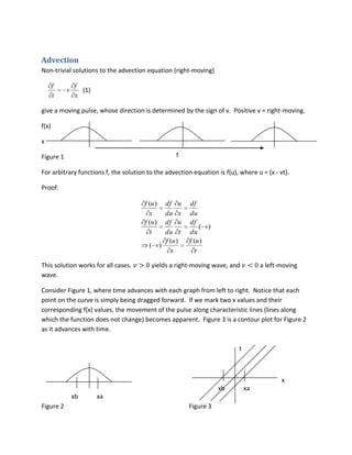
SlideShare a Scribd company logo
Advection<br />Non-trivial solutions to the advection equation (right-moving)<br />(1)<br />give a moving pulse, whose direction is determined by the sign of v.  Positive v = right-moving.<br />f(x)<br />tx<br />Figure 1<br />For arbitrary functions f, the solution to the advection equation is f(u), where u = (x - vt).<br />Proof:<br />This solution works for all cases. v>0 yields a right-moving wave, and v<0 a left-moving wave.<br />Consider Figure 1, where time advances with each graph from left to right.  Notice that each point on the curve is simply being dragged forward.  If we mark two x values and their corresponding f(x) values, the movement of the pulse along characteristic lines (lines along which the function does not change) becomes apparent.  Figure 3 is a contour plot for Figure 2 as it advances with time.<br />t<br />xb            xax<br />xb            xa<br />Figure 2Figure 3<br />Derivative Approximations<br />Forward Time Centered Space (FTCS) (Garcia 2000)<br />Consider a set of grid points with known x and f(x) values.  We will say this set of data points exists at time level t = tn, and xi denotes x at the ith place.  The distance between points is equal to Δx, and the duration between time levels is Δt. <br />What if we want to find information at another time level? (Figure 4)<br />fin+1?<br />Figure 4 finknown<br />We assume this data obeys the advection equation and estimate the function values at time level t = tn+1 using a forward time centered space approximation (FTCS).<br />Recall equation (1).<br />⇒∂f∂tx=xi,t=tn=-v∂f∂xx=xi,t=tn<br />The partial derivative on the right side of this equation can be approximated as<br />≈fi+1n- fi-1n2∆x<br />The partial derivative on the left as<br />≈fin+1- fin∆t<br />Equating the two with the appropriate constant v yields<br />fin+1- fin∆t=-vfi+1n- fi-1n2∆x<br />Solving for fin+1gives<br />fin+1=fin+fi+1n- fi-1n2∆x-v∆t      (2)<br />The approximation of the space derivative is second order accurate by virtue of being a centered derivative approximation.  The approximation of the time derivative is only first order accurate since it is a forward derivative approximation.<br />The computational molecule, which shows what points are used to approximate the value at the desired point, for FTCS is<br />Figure 5<br />FTCS is unconditionally unstable. If allowed to run for long enough, an FTCS algorithm will always blow up – infinities will start to show up in later time steps.<br />In most numerical methods for evolving hyperbolic partial differential equations, the stability of the system is determined by the Courant factor. The courant factor is α=v∆t∆x, or the ratio of physical wave speed to the speed at which the algorithm propagates information.<br />tConsider a physical light cone.<br />x<br />Figure 6<br />Only events within in the light cone can influence or be influenced by an observer at the origin.  For our purposes, the physical light cone of the wave is determined by the physical speed of the wave.  The numerical light cone is determined by the spacing of the grid on which function values are known.  For example, looking at the computational molecule for FTCS, you can see that numerical light cone.<br />Figure 7<br />Computationally, the only information affecting the approximation of the function value at the gray point is the information at the three black points. Consider a physical light cone mapped onto Figure 7.<br />Figure 8<br />Here, the physical light cone is smaller than the numerical light cone because v<ΔxΔt.  Stable approximations will have a numerical light cone bigger than a physical light cone, or a Courant factor α≤1.  Keeping with the physical light cone analogy (Figure 6), the computational system can be understood heuristically as taking into account all possible physical influences.  However, recall that FTCS is unconditionally unstable, and will eventually blow up even when this condition is satisfied.  <br />To get an idea of the problems with FTCS, consider a simple situation such as when a Courant factor is α=1. Here, we would expect that this algorithm would essentially drag the pulse along characteristic lines.  This is not true for FTCS.  Recall equation (2).<br />fin+1=fin+fi+1n- fi-1n2∆x-v∆t <br />For a Courant factor α=1, the algorithm becomes<br />fin+1=fin-fi+1n- fi-1n2     (3)<br />Since we have provided the algorithm with a very simple system and are looking at a symmetric situation that it should be able to handle easily, we should expect a rather clean-looking answer like <br />fin+1=fi-1n     (4)<br />In the case of equation (4), the wave is simply pulled along the characteristic line, which is what should happen computationally when numerical and physical speeds are equal; however, this is clearly not the case for FTCS.  Although this is not a rigorous explanation for the fact that FTCS is unconditionally unstable, it does show some of the issues with using FTCS, even when solving very simple systems.<br />Lax (Garcia 2000)<br />Instead of using a known data point at (xi,tn)and then adding the time derivative multiplied by ∆t(-v), the Lax method uses an average of the two points adjacent to xi at time level tnThe lax method uses the average of points to find the point at the next time step.<br />Average <br />Figure 11<br />fin+1=12fi+1n+ fi-1n+ ∆t-vfi+1n- fi-1n2∆x       (7)<br />The Lax method includes a diffusion term, which acts as though it takes energy away from the wave, preventing it from blowing up to infinity.  As is expected, the Lax method becomes unstable with large Courant factors, but it will also become unstable with very small Courant factors.  In the latter condition, the pulse dissipates rather quickly.<br />Centered Time Centered Space (Garcia 2000)<br />The Centered Time Centered Space method uses two initial time levels of data in order to get centered derivatives that are second-order accurate in both space and time <br />n<br />Figure 9<br />From before<br />-v∂f∂xx=xi,t=tn=∂f∂tx=xi,t=tn       (5)<br />The derivative approximations are<br />∂f∂xx=xi,t=tn≈fi+1n-fi-1n2∆x<br />And<br />∂f∂tx=xi,t=tn≈fin+1-fin-12∆t<br />Solving equation (5) yields<br />fin+1=fin-1+fi+1n- fi-1n∆x-v∆t      (6)<br />Note that the computational molecule for CTCS is<br />Figure 10<br />If α=1, we can assume within a reasonable uncertainty that fin-1 = fi+1n.  Therefore, equation (6) reduces to fin+1≈fi-1n.  This becomes exact if initial data ensures that fi'=fi+12.<br />Lax-Wendroff (Garcia 2000)<br />This method finds second derivatives, which it then uses to get to the next time step. Figure 12 provides a graphical representation of estimating second derivatives.  The derivative is being approximated at the center black point.<br />∂f∂x∂f∂x<br />∂2f∂x2<br />Figure 12<br />Consider a Taylor series expansion<br />ft+∆t,x=f(t,x)+∆t∂f∂tt,x+∆t22!∂2f∂tt,x+…<br />The  FTCS effectively truncates the Taylor series estimation at the term with the first-order partial differential.  Lax-Wendroff carries the estimation one term further in the expansion. <br />An alternative way of using the Lax-Wendroff method takes a lax step to an intermediate time level and then “leaps” across that intermediate step to the desired value.<br />643Black dots = initial data21<br />5<br />Figure 12<br />For each step in Figure 12:<br />,[object Object]
∂f∂xx=xi+12,t=tn≈fi+1n-fin∆x
fi-12n+12≈fi-1n + fin2+∆t2fin- fi-1n∆x-v
fi+12n+12≈fin + fi+1n2+∆t2fi+1n- fin∆x-v
∂f∂xx=xi,t=tn+12≈fi+12n+12-fi-12n+12∆x
fin+1≈∆t(v)2∆x+∆t2v22∆x2fi-1n+1-∆t2v2∆x2fin+∆t(-v)2∆x+∆t2v22∆x2fi+1nLax-Wendroff is essentially FTCS plus a diffusion term.  Although the difference between FTCS and Lax-Wendroff is basically a matter of an additional term, Lax-Wendroff is stable for the Courant condition α≤1 and is second-order accurate in both time and space.  This method does suffer from a dissipation problem similar to the Lax method. However, Lax-Wendroff is not affected as greatly by this issue as Lax is.<br />Iterated Crank-Nicholson (Teukolsky 2008)<br />The iterated Crank-Nicholson method makes a guess at the values of the next time step and then improves the guess by averaging.  This method is stable for 4n+2 and 4n+3 iterations where n = 0,1,2,3,… However, doing more than two corrections is not really helpful.<br />Consider the advection equation (1) without the velocity factor.<br />FTCS gives<br />fin+1-fin∆t=fi+1n-fi-1n2∆x<br />Backwards differencing (which is unconditionally stable) gives<br />fin+1-fin∆t=fi+1n+1-fi-1n+12∆x     (8)<br />Crank-Nicholson averages these two methods.<br />The first iteration of Crank-Nicholson calculates an intermediate variable using FTCS:<br />fin+1-fin∆t=fi+1n-fi-1n2∆x      (9)<br />Another intermediate variable is found by averaging<br />fin+12=12fin+1+fin         (10)<br />Then the time step is made using f in an FTCS approximation<br />fin+1-fin∆t=fi+1n+12-fi-1n+122∆x     (11)<br />A two-step iteration is done the same way.  After equations (9) and (10):<br />fin+1-fin∆t=fi+1n+12-fi-1n+122∆x     (12)<br />fin+12=12fin+1+fin<br />The time step is then made as in equation (12).<br />fin+1-fin∆t=fi+1n+12-fi-1n+122∆x     (13)<br />As shown by Teukolsky, 2008, Crank-Nicholson is stable for courant factors α≤2, or α24≤1.  <br />Upwind Method (Garcia 2000)<br />This method exploits the directionality of the wave by using only points that would trail the wave (physically) in the calculations. One benefit of this method is that we need only provide a boundary condition for the side of the computational domain away from which the wave travels. The computational molecule for this method is<br />Figure 13<br />And its numerical light cone is<br />Figure 14<br />The algorithm for a right-moving pulse, obeying the advection equation is<br />fin=fin-1-v∆t∆xfin-1-fi-1n-1       (14)<br />At the left boundary, some known value is provided (e.g., constant at 0) at each time step.  Providing known values as boundaries is known as Drichlet boundary conditions.  A right boundary condition is not necessary as the wave will simply move off the edge of the computational world – outgoing boundary condition.  For a left-moving pulse, we would simply need to mirror the points used (e.g., fin becomes the left-most point for a given set rather than the right-most).<br />Beam-Warming (Dullemond and Kuiper 2008)<br />Whereas the upwind method only used two points at the previous time level (Figure 13), the Beam-Warming method uses three.<br />Figure 15<br />The partial differential equation (PDE) for the Beam-Warming method looks something like<br />∂f∂t=v∂f∂xx=xi+12,t=tn-v2∂2f∂x2x=xi+1,t=tn       (15)<br />The second derivative term is a diffusion term, which acts as if it is taking energy away from the pulse, preventing it from blowing up.  The right-moving algorithm for this method is<br />fin+1=1-3v∆t2∆x+v2∆t22∆x2fin+2v∆t∆x-v2∆t2∆x2fi-1n+(-v)∆t2∆x+v2∆t22∆x2fi-1n     (16)<br />Again, these points can simply be mirrored for a left-moving algorithm. Also, note that this system requires boundary conditions for the two left-most points, whereas upwind only needed a boundary condition for the one, left-most point.<br />Box Method<br />The Box method uses two points at the previous time step and one point on the current time step in order to approximate a point at the current time step.<br />in-1<br />Figure 16<br />The PDE for the Box method is<br />-v∂f∂xx=xi-12,t=tn-1-v∂f∂xx=xi-12,t=tn2=∂f∂tx=xi,t=tn-12+∂f∂tx=xi-1,t=tn-122       (17)<br />The algorithm is<br />fin=fi-1n-1+fin-1-fi-1nv∆t-∆xv∆t+∆x      <br />Recall that <br />α=v∆t∆x<br />So, the algorithm can be reduced to<br />fin=fi-1n-1+fin-1-fi-1n1-α1+α     (18)  <br />Note the numerical light cone for this system<br />Figure 17<br />Because the light cone encompasses all previous points at all previous time levels, this system should be stable even for very large Courant factors.<br />Wave Equation<br />The simplest one-dimensional wave equation is<br />(19).<br />This equation has the solution f(u), where u  = x + vt or x – vt.<br />Proof:<br />Show that f(u) where u = x + vt is a solution to equation 2.<br />1st partial<br />2nd partial<br />1st partial<br />2nd partial<br />The proof for u = x – vt is similar.  Also, it has already been shown that characteristics have velocities ±v.<br />Crank Nicholson and the Wave Equation<br />Recall the wave equation (19).<br />In two-variable form, this equation is.<br />∂f∂t=ft         ∂ft∂t=v2∂2y∂x2        (20)<br />We can discretize this equation using Crank-Nicholson.  However, we need two pieces of initial data. Either f and ft at one time level or f at two time levels.  For discretization, I will assume the first situation, with known values at time level t = tn-1.<br />fin-fin-1∆t=ftin-1<br />ftin-ftin-1∆t=v2fi+1n-1-2fin-1+fi-1n-1∆x2<br />fin-fin-1∆t=ftin-12=ftin-1+ftin2<br />ftin-ftin-1∆t=v2fi+1n-12-2fin-12+fi-1n-12∆x2<br />Note that here fin-12=fin+fin-12<br />fin-fin-1∆t=ftin-12=ftin-1+ftin2<br />ftin-ftin-1∆t=v2fi+1n-12-2fin-12+fi-1n-12∆x2<br />Note that here fin-12=fin+fin-12<br />Boundary Conditions for the Wave Equation<br />From the section on approximating numerical derivative, the Upwind, Beam-Warming, and Box methods are particularly useful for establishing boundary conditions.<br />When a wave is evolved forward in time numerically, the system doing the evolution loses information at the boundaries of the domain over which the wave is being evolved.<br />Information lost at boundariesTime advances  <br />Numerical Domain<br />Figure 18<br />Consider the wave equation (19)<br />This equation has as a solution <br />fx,t= Fx-vt+ Gx+vt      (21)<br />The F term is the right-moving part of the wave and the G term is the left-moving part.  These two parts are independently both solutions of the advection equation (1).<br />∂F∂t=-v∂F∂x           ∂G∂t=v∂G∂x<br />Therefore, we can use the aforementioned methods for boundary conditions by forcing the wave equation to obey the appropriate advection equation (left-moving or right-moving) at the boundaries.<br />Wave equation in Spherical Coordinates<br />The three dimensional wave equation in spherical coordinates is<br />∂2f∂t2=v2∇2f     (22)<br />The Laplacian in spherical coordinates is<br />∇2f=1r2∂∂rr2∂f∂r+1rrsinθ∂∂θsinθ∂f∂θ+1r2sinθ∂2f∂ϕ2      23<br />If f=f(r,t)<br />∂f∂θ=0  &  ∂f∂ϕ=0<br />The Laplacian reduces to <br />∇2f(r,t)=1r2∂∂rr2∂f∂r<br />So<br />∂2f∂t2=v21r2∂∂rr2∂f∂r<br />∂2f∂t2=v2∂2f∂r2+2r∂f∂r        (24)<br />Note that at the origin, the 2r∂f∂r term will be zero, because ∂f∂r is 0 at the origin.<br />Boundary Conditions for the Wave Equation in 3-D<br />Outgoing Boundary<br />Recall that solutions to the wave equation (19) have left and right moving parts that obey the advection equation.  See equation (21), copied here.<br />fx,t= Fx-vt+ Gx+vt <br />However, the 3-D wave equation in spherical coordinates (24) has an additional term.<br />∂2f∂t2=v2∂2f∂r2+2r∂f∂r <br />How can we use our out-going boundary conditions (Upwind, Beam-Warming, and Box) with a 3-D wave equation?<br />Letg=(r±vt)<br />That is to say,∂g∂t=±v∂g∂r<br />Also, letfr=hrg(r+ϵvt)<br />Where ϵ=±1<br />Recalling that∂2f∂t2=v21r2∂∂rr2∂f∂r<br />Find hr that makes this work.<br />∂f∂t=hg'ϵv<br />∂f∂r=h'g+hg'<br />∂2f∂t2=hg''ϵv2<br />∂2f∂r2=h''g+g'h'+h'g'+hg''=h''g+2h'g'+hg''<br />∂2f∂t2=v2∂2f∂r2+2r∂f∂r<br />v2hg''=v2(h''g+2h'g'+hg''+2rh'g+2rhg'<br />0=h''+2rh'g+2h'+1rhg'<br />h''= -2rh      h'=-1rh<br />Now all we have to do is solve the ODE<br />dhdr=-hr<br />dhh=-drr<br />h=cr<br />Now,<br />ft,r=gr±vtr<br />∂∂trf=-v∂∂rrf<br />Considering the previous boundary conditions, such as the box method, all that needs to change is f⇒rf.<br />For example, the Box method algorithm (18) becomes<br />rifin=ri-1fi-1n-1+rifin-1-ri-1 fi-1n1-α1+α<br />In short, rf obeys a simpler wave equation.<br />Boundary at the Origin<br />Findf'0r<br />At the origin<br />limr->0f'rr<br />Consider the Taylor series<br />f(r)=f(0)+rf'(0)1!+r2f''(0)2!+r3f'''(0)3!+…<br />So, we can see that<br />limr->0f'rr=limr->0f0+rf'01!+r2f''02!+r3f'''03!+…=f''0<br />Exploiting the fact that the wave is symmetric about the origin, the second derivative at the origin can easily be approximated as <br />∂2f∂r2≈2f∆r-f0∆r2   (25)<br />∂f∂r∂f∂r<br />∂2f∂r2<br />Figure 19<br />Also, by considering the Laplacian in Cartesian coordinates<br />∂2f∂t2=v2∂2f∂y2+∂2f∂y2+∂2f∂z2 <br />Due to the spherical symmetry about the origin (r=0),<br />∂2f∂x2=∂2f∂y2+∂2f∂z2<br />Therefore,<br />∂2f∂x2=3v2∂2f∂r2<br />Discretizing the Wave Equation<br />CFL<br />∂2f∂t2=v2∂2f∂r2+2r∂f∂r <br />fin+1-2fin+fin-1∆t2=v2f i-1n-2fin+fi+1n∆r2+2rfi+1n-fi-1n2∆r<br />At r = 0<br />∂2f∂t2=3v2∂2f∂22<br />At outer boundary<br />∂g∂t=-v ∂g∂r<br />Where g=fr<br />Crank-Nicholson<br />∂2f∂t2=v2∂2f∂r2+2r∂f∂r <br />Let∂f∂t=ft    ⇒    ∂ft∂t=v2∂2f∂r2+2r∂f∂r <br />fin-fin-1∆t=ftin-1<br />ftin-ftin-1∆t=v2fi+1n-1-2fin-1+fi-1n-1∆x2+2rfi+1n-1-fi-1n-12∆x<br />fin-fin-1∆t=ftin-12=ftin-1+ftin2<br />ftin-ftin-1∆t=v2fi+1n-12-2fin-12+fi-1n-12∆x2+2rfi+1n-12-fi-1n-122∆x<br />fin-fin-1∆t=ftin-12=ftin-1+ftin2<br />ftin-ftin-1∆t=v2fi+1n-12-2fin-12+fi-1n-12∆x2+2rfi+1 n-12-fi-1n-122x2<br />At r = 0<br />∂2f∂t2=3v2∂2f∂22<br />At outer boundary<br />∂g∂t=-v ∂g∂r<br />Where g=fr<br />
Physics Research Summer2009

More Related Content

What's hot

Mechanical Engineering Assignment Help
Mechanical Engineering Assignment HelpMechanical Engineering Assignment Help
Mechanical Engineering Assignment Help
Matlab Assignment Experts
 
DSP_FOEHU - MATLAB 02 - The Discrete-time Fourier Analysis
DSP_FOEHU - MATLAB 02 - The Discrete-time Fourier AnalysisDSP_FOEHU - MATLAB 02 - The Discrete-time Fourier Analysis
DSP_FOEHU - MATLAB 02 - The Discrete-time Fourier Analysis
Amr E. Mohamed
 
Computational Method to Solve the Partial Differential Equations (PDEs)
Computational Method to Solve the Partial Differential  Equations (PDEs)Computational Method to Solve the Partial Differential  Equations (PDEs)
Computational Method to Solve the Partial Differential Equations (PDEs)
Dr. Khurram Mehboob
 
Design of sampled data control systems part 2. 6th lecture
Design of sampled data control systems part 2.  6th lectureDesign of sampled data control systems part 2.  6th lecture
Design of sampled data control systems part 2. 6th lecture
Khalaf Gaeid Alshammery
 
Jensen's inequality, EM 알고리즘
Jensen's inequality, EM 알고리즘 Jensen's inequality, EM 알고리즘
Jensen's inequality, EM 알고리즘
Jungkyu Lee
 
DSP_FOEHU - MATLAB 01 - Discrete Time Signals and Systems
DSP_FOEHU - MATLAB 01 - Discrete Time Signals and SystemsDSP_FOEHU - MATLAB 01 - Discrete Time Signals and Systems
DSP_FOEHU - MATLAB 01 - Discrete Time Signals and Systems
Amr E. Mohamed
 
Approximate Methods
Approximate MethodsApproximate Methods
Approximate Methods
Teja Ande
 
Design of sampled data control systems 5th lecture
Design of sampled data control systems  5th  lectureDesign of sampled data control systems  5th  lecture
Design of sampled data control systems 5th lecture
Khalaf Gaeid Alshammery
 
Introduction to Fourier transform and signal analysis
Introduction to Fourier transform and signal analysisIntroduction to Fourier transform and signal analysis
Introduction to Fourier transform and signal analysis
宗翰 謝
 
Sienna 4 divideandconquer
Sienna 4 divideandconquerSienna 4 divideandconquer
Sienna 4 divideandconquerchidabdu
 
Stochastic Processes Homework Help
Stochastic Processes Homework Help Stochastic Processes Homework Help
Stochastic Processes Homework Help
Statistics Assignment Help
 
no U-turn sampler, a discussion of Hoffman & Gelman NUTS algorithm
no U-turn sampler, a discussion of Hoffman & Gelman NUTS algorithmno U-turn sampler, a discussion of Hoffman & Gelman NUTS algorithm
no U-turn sampler, a discussion of Hoffman & Gelman NUTS algorithm
Christian Robert
 
Dcs lec02 - z-transform
Dcs   lec02 - z-transformDcs   lec02 - z-transform
Dcs lec02 - z-transform
Amr E. Mohamed
 
Digital Signal Processing Assignment Help
Digital Signal Processing Assignment HelpDigital Signal Processing Assignment Help
Digital Signal Processing Assignment Help
Matlab Assignment Experts
 
Finite DIfference Methods Mathematica
Finite DIfference Methods MathematicaFinite DIfference Methods Mathematica
Finite DIfference Methods Mathematica
guest56708a
 
Fourier Series for Continuous Time & Discrete Time Signals
Fourier Series for Continuous Time & Discrete Time SignalsFourier Series for Continuous Time & Discrete Time Signals
Fourier Series for Continuous Time & Discrete Time Signals
Jayanshu Gundaniya
 
D I G I T A L C O N T R O L S Y S T E M S J N T U M O D E L P A P E R{Www
D I G I T A L  C O N T R O L  S Y S T E M S  J N T U  M O D E L  P A P E R{WwwD I G I T A L  C O N T R O L  S Y S T E M S  J N T U  M O D E L  P A P E R{Www
D I G I T A L C O N T R O L S Y S T E M S J N T U M O D E L P A P E R{Wwwguest3f9c6b
 
DSP 08 _ Sheet Eight
DSP 08 _ Sheet EightDSP 08 _ Sheet Eight
DSP 08 _ Sheet Eight
Amr E. Mohamed
 

What's hot (20)

Mechanical Engineering Assignment Help
Mechanical Engineering Assignment HelpMechanical Engineering Assignment Help
Mechanical Engineering Assignment Help
 
DSP_FOEHU - MATLAB 02 - The Discrete-time Fourier Analysis
DSP_FOEHU - MATLAB 02 - The Discrete-time Fourier AnalysisDSP_FOEHU - MATLAB 02 - The Discrete-time Fourier Analysis
DSP_FOEHU - MATLAB 02 - The Discrete-time Fourier Analysis
 
Computational Method to Solve the Partial Differential Equations (PDEs)
Computational Method to Solve the Partial Differential  Equations (PDEs)Computational Method to Solve the Partial Differential  Equations (PDEs)
Computational Method to Solve the Partial Differential Equations (PDEs)
 
Design of sampled data control systems part 2. 6th lecture
Design of sampled data control systems part 2.  6th lectureDesign of sampled data control systems part 2.  6th lecture
Design of sampled data control systems part 2. 6th lecture
 
Jensen's inequality, EM 알고리즘
Jensen's inequality, EM 알고리즘 Jensen's inequality, EM 알고리즘
Jensen's inequality, EM 알고리즘
 
DSP_FOEHU - MATLAB 01 - Discrete Time Signals and Systems
DSP_FOEHU - MATLAB 01 - Discrete Time Signals and SystemsDSP_FOEHU - MATLAB 01 - Discrete Time Signals and Systems
DSP_FOEHU - MATLAB 01 - Discrete Time Signals and Systems
 
Approximate Methods
Approximate MethodsApproximate Methods
Approximate Methods
 
1416336962.pdf
1416336962.pdf1416336962.pdf
1416336962.pdf
 
Design of sampled data control systems 5th lecture
Design of sampled data control systems  5th  lectureDesign of sampled data control systems  5th  lecture
Design of sampled data control systems 5th lecture
 
Introduction to Fourier transform and signal analysis
Introduction to Fourier transform and signal analysisIntroduction to Fourier transform and signal analysis
Introduction to Fourier transform and signal analysis
 
Sienna 4 divideandconquer
Sienna 4 divideandconquerSienna 4 divideandconquer
Sienna 4 divideandconquer
 
Stochastic Processes Homework Help
Stochastic Processes Homework Help Stochastic Processes Homework Help
Stochastic Processes Homework Help
 
no U-turn sampler, a discussion of Hoffman & Gelman NUTS algorithm
no U-turn sampler, a discussion of Hoffman & Gelman NUTS algorithmno U-turn sampler, a discussion of Hoffman & Gelman NUTS algorithm
no U-turn sampler, a discussion of Hoffman & Gelman NUTS algorithm
 
Dcs lec02 - z-transform
Dcs   lec02 - z-transformDcs   lec02 - z-transform
Dcs lec02 - z-transform
 
Digital Signal Processing Assignment Help
Digital Signal Processing Assignment HelpDigital Signal Processing Assignment Help
Digital Signal Processing Assignment Help
 
Finite DIfference Methods Mathematica
Finite DIfference Methods MathematicaFinite DIfference Methods Mathematica
Finite DIfference Methods Mathematica
 
Fourier Series for Continuous Time & Discrete Time Signals
Fourier Series for Continuous Time & Discrete Time SignalsFourier Series for Continuous Time & Discrete Time Signals
Fourier Series for Continuous Time & Discrete Time Signals
 
Fdtd
FdtdFdtd
Fdtd
 
D I G I T A L C O N T R O L S Y S T E M S J N T U M O D E L P A P E R{Www
D I G I T A L  C O N T R O L  S Y S T E M S  J N T U  M O D E L  P A P E R{WwwD I G I T A L  C O N T R O L  S Y S T E M S  J N T U  M O D E L  P A P E R{Www
D I G I T A L C O N T R O L S Y S T E M S J N T U M O D E L P A P E R{Www
 
DSP 08 _ Sheet Eight
DSP 08 _ Sheet EightDSP 08 _ Sheet Eight
DSP 08 _ Sheet Eight
 

Similar to Physics Research Summer2009

Conjugate Gradient Methods
Conjugate Gradient MethodsConjugate Gradient Methods
Conjugate Gradient Methods
MTiti1
 
S3-3.pdf
S3-3.pdfS3-3.pdf
S3-3.pdf
MuhammadSajed1
 
Synchronizing Chaotic Systems - Karl Dutson
Synchronizing Chaotic Systems - Karl DutsonSynchronizing Chaotic Systems - Karl Dutson
Synchronizing Chaotic Systems - Karl DutsonKarl Dutson
 
Newton_Rapson method.pdf
Newton_Rapson method.pdfNewton_Rapson method.pdf
Newton_Rapson method.pdf
SandaruwanChathurang2
 
Newton's Raphson method
Newton's Raphson methodNewton's Raphson method
Newton's Raphson method
Saloni Singhal
 
Secant method
Secant methodSecant method
Secant method
Zahra Saman
 
SURF 2012 Final Report(1)
SURF 2012 Final Report(1)SURF 2012 Final Report(1)
SURF 2012 Final Report(1)Eric Zhang
 
WaveletTutorial.pdf
WaveletTutorial.pdfWaveletTutorial.pdf
WaveletTutorial.pdf
shreyassr9
 
Online Signals and Systems Assignment Help
Online Signals and Systems Assignment HelpOnline Signals and Systems Assignment Help
Online Signals and Systems Assignment Help
Matlab Assignment Experts
 
App8
App8App8
Numerical Methods
Numerical MethodsNumerical Methods
Numerical Methods
Teja Ande
 
Fourier Specturm via MATLAB
Fourier Specturm via MATLABFourier Specturm via MATLAB
Fourier Specturm via MATLABZunAib Ali
 
Decision directed carrier signal
Decision directed carrier signalDecision directed carrier signal
Decision directed carrier signal
sunil kumar
 
Quadrature
QuadratureQuadrature
Quadrature
Linh Tran
 
What are free particles in quantum mechanics
What are free particles in quantum mechanicsWhat are free particles in quantum mechanics
What are free particles in quantum mechanics
bhaskar chatterjee
 
A multiphase lattice Boltzmann model with sharp interfaces
A multiphase lattice Boltzmann model with sharp interfacesA multiphase lattice Boltzmann model with sharp interfaces
A multiphase lattice Boltzmann model with sharp interfaces
Tim Reis
 
Stochastic Processes Assignment Help
Stochastic Processes Assignment HelpStochastic Processes Assignment Help
Stochastic Processes Assignment Help
Statistics Assignment Help
 

Similar to Physics Research Summer2009 (20)

Conjugate Gradient Methods
Conjugate Gradient MethodsConjugate Gradient Methods
Conjugate Gradient Methods
 
S3-3.pdf
S3-3.pdfS3-3.pdf
S3-3.pdf
 
Synchronizing Chaotic Systems - Karl Dutson
Synchronizing Chaotic Systems - Karl DutsonSynchronizing Chaotic Systems - Karl Dutson
Synchronizing Chaotic Systems - Karl Dutson
 
Newton_Rapson method.pdf
Newton_Rapson method.pdfNewton_Rapson method.pdf
Newton_Rapson method.pdf
 
Newton's Raphson method
Newton's Raphson methodNewton's Raphson method
Newton's Raphson method
 
Secant method
Secant methodSecant method
Secant method
 
SURF 2012 Final Report(1)
SURF 2012 Final Report(1)SURF 2012 Final Report(1)
SURF 2012 Final Report(1)
 
AJMS_389_22.pdf
AJMS_389_22.pdfAJMS_389_22.pdf
AJMS_389_22.pdf
 
WaveletTutorial.pdf
WaveletTutorial.pdfWaveletTutorial.pdf
WaveletTutorial.pdf
 
Online Signals and Systems Assignment Help
Online Signals and Systems Assignment HelpOnline Signals and Systems Assignment Help
Online Signals and Systems Assignment Help
 
App8
App8App8
App8
 
Numerical Methods
Numerical MethodsNumerical Methods
Numerical Methods
 
Fourier Specturm via MATLAB
Fourier Specturm via MATLABFourier Specturm via MATLAB
Fourier Specturm via MATLAB
 
Decision directed carrier signal
Decision directed carrier signalDecision directed carrier signal
Decision directed carrier signal
 
Ch02
Ch02Ch02
Ch02
 
Ch02
Ch02Ch02
Ch02
 
Quadrature
QuadratureQuadrature
Quadrature
 
What are free particles in quantum mechanics
What are free particles in quantum mechanicsWhat are free particles in quantum mechanics
What are free particles in quantum mechanics
 
A multiphase lattice Boltzmann model with sharp interfaces
A multiphase lattice Boltzmann model with sharp interfacesA multiphase lattice Boltzmann model with sharp interfaces
A multiphase lattice Boltzmann model with sharp interfaces
 
Stochastic Processes Assignment Help
Stochastic Processes Assignment HelpStochastic Processes Assignment Help
Stochastic Processes Assignment Help
 

Recently uploaded

Empowering NextGen Mobility via Large Action Model Infrastructure (LAMI): pav...
Empowering NextGen Mobility via Large Action Model Infrastructure (LAMI): pav...Empowering NextGen Mobility via Large Action Model Infrastructure (LAMI): pav...
Empowering NextGen Mobility via Large Action Model Infrastructure (LAMI): pav...
Thierry Lestable
 
FIDO Alliance Osaka Seminar: Passkeys at Amazon.pdf
FIDO Alliance Osaka Seminar: Passkeys at Amazon.pdfFIDO Alliance Osaka Seminar: Passkeys at Amazon.pdf
FIDO Alliance Osaka Seminar: Passkeys at Amazon.pdf
FIDO Alliance
 
From Siloed Products to Connected Ecosystem: Building a Sustainable and Scala...
From Siloed Products to Connected Ecosystem: Building a Sustainable and Scala...From Siloed Products to Connected Ecosystem: Building a Sustainable and Scala...
From Siloed Products to Connected Ecosystem: Building a Sustainable and Scala...
Product School
 
PHP Frameworks: I want to break free (IPC Berlin 2024)
PHP Frameworks: I want to break free (IPC Berlin 2024)PHP Frameworks: I want to break free (IPC Berlin 2024)
PHP Frameworks: I want to break free (IPC Berlin 2024)
Ralf Eggert
 
The Art of the Pitch: WordPress Relationships and Sales
The Art of the Pitch: WordPress Relationships and SalesThe Art of the Pitch: WordPress Relationships and Sales
The Art of the Pitch: WordPress Relationships and Sales
Laura Byrne
 
GenAISummit 2024 May 28 Sri Ambati Keynote: AGI Belongs to The Community in O...
GenAISummit 2024 May 28 Sri Ambati Keynote: AGI Belongs to The Community in O...GenAISummit 2024 May 28 Sri Ambati Keynote: AGI Belongs to The Community in O...
GenAISummit 2024 May 28 Sri Ambati Keynote: AGI Belongs to The Community in O...
Sri Ambati
 
Dev Dives: Train smarter, not harder – active learning and UiPath LLMs for do...
Dev Dives: Train smarter, not harder – active learning and UiPath LLMs for do...Dev Dives: Train smarter, not harder – active learning and UiPath LLMs for do...
Dev Dives: Train smarter, not harder – active learning and UiPath LLMs for do...
UiPathCommunity
 
IOS-PENTESTING-BEGINNERS-PRACTICAL-GUIDE-.pptx
IOS-PENTESTING-BEGINNERS-PRACTICAL-GUIDE-.pptxIOS-PENTESTING-BEGINNERS-PRACTICAL-GUIDE-.pptx
IOS-PENTESTING-BEGINNERS-PRACTICAL-GUIDE-.pptx
Abida Shariff
 
Neuro-symbolic is not enough, we need neuro-*semantic*
Neuro-symbolic is not enough, we need neuro-*semantic*Neuro-symbolic is not enough, we need neuro-*semantic*
Neuro-symbolic is not enough, we need neuro-*semantic*
Frank van Harmelen
 
Epistemic Interaction - tuning interfaces to provide information for AI support
Epistemic Interaction - tuning interfaces to provide information for AI supportEpistemic Interaction - tuning interfaces to provide information for AI support
Epistemic Interaction - tuning interfaces to provide information for AI support
Alan Dix
 
Software Delivery At the Speed of AI: Inflectra Invests In AI-Powered Quality
Software Delivery At the Speed of AI: Inflectra Invests In AI-Powered QualitySoftware Delivery At the Speed of AI: Inflectra Invests In AI-Powered Quality
Software Delivery At the Speed of AI: Inflectra Invests In AI-Powered Quality
Inflectra
 
Leading Change strategies and insights for effective change management pdf 1.pdf
Leading Change strategies and insights for effective change management pdf 1.pdfLeading Change strategies and insights for effective change management pdf 1.pdf
Leading Change strategies and insights for effective change management pdf 1.pdf
OnBoard
 
De-mystifying Zero to One: Design Informed Techniques for Greenfield Innovati...
De-mystifying Zero to One: Design Informed Techniques for Greenfield Innovati...De-mystifying Zero to One: Design Informed Techniques for Greenfield Innovati...
De-mystifying Zero to One: Design Informed Techniques for Greenfield Innovati...
Product School
 
Key Trends Shaping the Future of Infrastructure.pdf
Key Trends Shaping the Future of Infrastructure.pdfKey Trends Shaping the Future of Infrastructure.pdf
Key Trends Shaping the Future of Infrastructure.pdf
Cheryl Hung
 
Bits & Pixels using AI for Good.........
Bits & Pixels using AI for Good.........Bits & Pixels using AI for Good.........
Bits & Pixels using AI for Good.........
Alison B. Lowndes
 
FIDO Alliance Osaka Seminar: Passkeys and the Road Ahead.pdf
FIDO Alliance Osaka Seminar: Passkeys and the Road Ahead.pdfFIDO Alliance Osaka Seminar: Passkeys and the Road Ahead.pdf
FIDO Alliance Osaka Seminar: Passkeys and the Road Ahead.pdf
FIDO Alliance
 
FIDO Alliance Osaka Seminar: FIDO Security Aspects.pdf
FIDO Alliance Osaka Seminar: FIDO Security Aspects.pdfFIDO Alliance Osaka Seminar: FIDO Security Aspects.pdf
FIDO Alliance Osaka Seminar: FIDO Security Aspects.pdf
FIDO Alliance
 
UiPath Test Automation using UiPath Test Suite series, part 3
UiPath Test Automation using UiPath Test Suite series, part 3UiPath Test Automation using UiPath Test Suite series, part 3
UiPath Test Automation using UiPath Test Suite series, part 3
DianaGray10
 
LF Energy Webinar: Electrical Grid Modelling and Simulation Through PowSyBl -...
LF Energy Webinar: Electrical Grid Modelling and Simulation Through PowSyBl -...LF Energy Webinar: Electrical Grid Modelling and Simulation Through PowSyBl -...
LF Energy Webinar: Electrical Grid Modelling and Simulation Through PowSyBl -...
DanBrown980551
 
To Graph or Not to Graph Knowledge Graph Architectures and LLMs
To Graph or Not to Graph Knowledge Graph Architectures and LLMsTo Graph or Not to Graph Knowledge Graph Architectures and LLMs
To Graph or Not to Graph Knowledge Graph Architectures and LLMs
Paul Groth
 

Recently uploaded (20)

Empowering NextGen Mobility via Large Action Model Infrastructure (LAMI): pav...
Empowering NextGen Mobility via Large Action Model Infrastructure (LAMI): pav...Empowering NextGen Mobility via Large Action Model Infrastructure (LAMI): pav...
Empowering NextGen Mobility via Large Action Model Infrastructure (LAMI): pav...
 
FIDO Alliance Osaka Seminar: Passkeys at Amazon.pdf
FIDO Alliance Osaka Seminar: Passkeys at Amazon.pdfFIDO Alliance Osaka Seminar: Passkeys at Amazon.pdf
FIDO Alliance Osaka Seminar: Passkeys at Amazon.pdf
 
From Siloed Products to Connected Ecosystem: Building a Sustainable and Scala...
From Siloed Products to Connected Ecosystem: Building a Sustainable and Scala...From Siloed Products to Connected Ecosystem: Building a Sustainable and Scala...
From Siloed Products to Connected Ecosystem: Building a Sustainable and Scala...
 
PHP Frameworks: I want to break free (IPC Berlin 2024)
PHP Frameworks: I want to break free (IPC Berlin 2024)PHP Frameworks: I want to break free (IPC Berlin 2024)
PHP Frameworks: I want to break free (IPC Berlin 2024)
 
The Art of the Pitch: WordPress Relationships and Sales
The Art of the Pitch: WordPress Relationships and SalesThe Art of the Pitch: WordPress Relationships and Sales
The Art of the Pitch: WordPress Relationships and Sales
 
GenAISummit 2024 May 28 Sri Ambati Keynote: AGI Belongs to The Community in O...
GenAISummit 2024 May 28 Sri Ambati Keynote: AGI Belongs to The Community in O...GenAISummit 2024 May 28 Sri Ambati Keynote: AGI Belongs to The Community in O...
GenAISummit 2024 May 28 Sri Ambati Keynote: AGI Belongs to The Community in O...
 
Dev Dives: Train smarter, not harder – active learning and UiPath LLMs for do...
Dev Dives: Train smarter, not harder – active learning and UiPath LLMs for do...Dev Dives: Train smarter, not harder – active learning and UiPath LLMs for do...
Dev Dives: Train smarter, not harder – active learning and UiPath LLMs for do...
 
IOS-PENTESTING-BEGINNERS-PRACTICAL-GUIDE-.pptx
IOS-PENTESTING-BEGINNERS-PRACTICAL-GUIDE-.pptxIOS-PENTESTING-BEGINNERS-PRACTICAL-GUIDE-.pptx
IOS-PENTESTING-BEGINNERS-PRACTICAL-GUIDE-.pptx
 
Neuro-symbolic is not enough, we need neuro-*semantic*
Neuro-symbolic is not enough, we need neuro-*semantic*Neuro-symbolic is not enough, we need neuro-*semantic*
Neuro-symbolic is not enough, we need neuro-*semantic*
 
Epistemic Interaction - tuning interfaces to provide information for AI support
Epistemic Interaction - tuning interfaces to provide information for AI supportEpistemic Interaction - tuning interfaces to provide information for AI support
Epistemic Interaction - tuning interfaces to provide information for AI support
 
Software Delivery At the Speed of AI: Inflectra Invests In AI-Powered Quality
Software Delivery At the Speed of AI: Inflectra Invests In AI-Powered QualitySoftware Delivery At the Speed of AI: Inflectra Invests In AI-Powered Quality
Software Delivery At the Speed of AI: Inflectra Invests In AI-Powered Quality
 
Leading Change strategies and insights for effective change management pdf 1.pdf
Leading Change strategies and insights for effective change management pdf 1.pdfLeading Change strategies and insights for effective change management pdf 1.pdf
Leading Change strategies and insights for effective change management pdf 1.pdf
 
De-mystifying Zero to One: Design Informed Techniques for Greenfield Innovati...
De-mystifying Zero to One: Design Informed Techniques for Greenfield Innovati...De-mystifying Zero to One: Design Informed Techniques for Greenfield Innovati...
De-mystifying Zero to One: Design Informed Techniques for Greenfield Innovati...
 
Key Trends Shaping the Future of Infrastructure.pdf
Key Trends Shaping the Future of Infrastructure.pdfKey Trends Shaping the Future of Infrastructure.pdf
Key Trends Shaping the Future of Infrastructure.pdf
 
Bits & Pixels using AI for Good.........
Bits & Pixels using AI for Good.........Bits & Pixels using AI for Good.........
Bits & Pixels using AI for Good.........
 
FIDO Alliance Osaka Seminar: Passkeys and the Road Ahead.pdf
FIDO Alliance Osaka Seminar: Passkeys and the Road Ahead.pdfFIDO Alliance Osaka Seminar: Passkeys and the Road Ahead.pdf
FIDO Alliance Osaka Seminar: Passkeys and the Road Ahead.pdf
 
FIDO Alliance Osaka Seminar: FIDO Security Aspects.pdf
FIDO Alliance Osaka Seminar: FIDO Security Aspects.pdfFIDO Alliance Osaka Seminar: FIDO Security Aspects.pdf
FIDO Alliance Osaka Seminar: FIDO Security Aspects.pdf
 
UiPath Test Automation using UiPath Test Suite series, part 3
UiPath Test Automation using UiPath Test Suite series, part 3UiPath Test Automation using UiPath Test Suite series, part 3
UiPath Test Automation using UiPath Test Suite series, part 3
 
LF Energy Webinar: Electrical Grid Modelling and Simulation Through PowSyBl -...
LF Energy Webinar: Electrical Grid Modelling and Simulation Through PowSyBl -...LF Energy Webinar: Electrical Grid Modelling and Simulation Through PowSyBl -...
LF Energy Webinar: Electrical Grid Modelling and Simulation Through PowSyBl -...
 
To Graph or Not to Graph Knowledge Graph Architectures and LLMs
To Graph or Not to Graph Knowledge Graph Architectures and LLMsTo Graph or Not to Graph Knowledge Graph Architectures and LLMs
To Graph or Not to Graph Knowledge Graph Architectures and LLMs
 

Physics Research Summer2009

  • 1.
  • 6. fin+1≈∆t(v)2∆x+∆t2v22∆x2fi-1n+1-∆t2v2∆x2fin+∆t(-v)2∆x+∆t2v22∆x2fi+1nLax-Wendroff is essentially FTCS plus a diffusion term. Although the difference between FTCS and Lax-Wendroff is basically a matter of an additional term, Lax-Wendroff is stable for the Courant condition α≤1 and is second-order accurate in both time and space. This method does suffer from a dissipation problem similar to the Lax method. However, Lax-Wendroff is not affected as greatly by this issue as Lax is.<br />Iterated Crank-Nicholson (Teukolsky 2008)<br />The iterated Crank-Nicholson method makes a guess at the values of the next time step and then improves the guess by averaging. This method is stable for 4n+2 and 4n+3 iterations where n = 0,1,2,3,… However, doing more than two corrections is not really helpful.<br />Consider the advection equation (1) without the velocity factor.<br />FTCS gives<br />fin+1-fin∆t=fi+1n-fi-1n2∆x<br />Backwards differencing (which is unconditionally stable) gives<br />fin+1-fin∆t=fi+1n+1-fi-1n+12∆x (8)<br />Crank-Nicholson averages these two methods.<br />The first iteration of Crank-Nicholson calculates an intermediate variable using FTCS:<br />fin+1-fin∆t=fi+1n-fi-1n2∆x (9)<br />Another intermediate variable is found by averaging<br />fin+12=12fin+1+fin (10)<br />Then the time step is made using f in an FTCS approximation<br />fin+1-fin∆t=fi+1n+12-fi-1n+122∆x (11)<br />A two-step iteration is done the same way. After equations (9) and (10):<br />fin+1-fin∆t=fi+1n+12-fi-1n+122∆x (12)<br />fin+12=12fin+1+fin<br />The time step is then made as in equation (12).<br />fin+1-fin∆t=fi+1n+12-fi-1n+122∆x (13)<br />As shown by Teukolsky, 2008, Crank-Nicholson is stable for courant factors α≤2, or α24≤1. <br />Upwind Method (Garcia 2000)<br />This method exploits the directionality of the wave by using only points that would trail the wave (physically) in the calculations. One benefit of this method is that we need only provide a boundary condition for the side of the computational domain away from which the wave travels. The computational molecule for this method is<br />Figure 13<br />And its numerical light cone is<br />Figure 14<br />The algorithm for a right-moving pulse, obeying the advection equation is<br />fin=fin-1-v∆t∆xfin-1-fi-1n-1 (14)<br />At the left boundary, some known value is provided (e.g., constant at 0) at each time step. Providing known values as boundaries is known as Drichlet boundary conditions. A right boundary condition is not necessary as the wave will simply move off the edge of the computational world – outgoing boundary condition. For a left-moving pulse, we would simply need to mirror the points used (e.g., fin becomes the left-most point for a given set rather than the right-most).<br />Beam-Warming (Dullemond and Kuiper 2008)<br />Whereas the upwind method only used two points at the previous time level (Figure 13), the Beam-Warming method uses three.<br />Figure 15<br />The partial differential equation (PDE) for the Beam-Warming method looks something like<br />∂f∂t=v∂f∂xx=xi+12,t=tn-v2∂2f∂x2x=xi+1,t=tn (15)<br />The second derivative term is a diffusion term, which acts as if it is taking energy away from the pulse, preventing it from blowing up. The right-moving algorithm for this method is<br />fin+1=1-3v∆t2∆x+v2∆t22∆x2fin+2v∆t∆x-v2∆t2∆x2fi-1n+(-v)∆t2∆x+v2∆t22∆x2fi-1n (16)<br />Again, these points can simply be mirrored for a left-moving algorithm. Also, note that this system requires boundary conditions for the two left-most points, whereas upwind only needed a boundary condition for the one, left-most point.<br />Box Method<br />The Box method uses two points at the previous time step and one point on the current time step in order to approximate a point at the current time step.<br />in-1<br />Figure 16<br />The PDE for the Box method is<br />-v∂f∂xx=xi-12,t=tn-1-v∂f∂xx=xi-12,t=tn2=∂f∂tx=xi,t=tn-12+∂f∂tx=xi-1,t=tn-122 (17)<br />The algorithm is<br />fin=fi-1n-1+fin-1-fi-1nv∆t-∆xv∆t+∆x <br />Recall that <br />α=v∆t∆x<br />So, the algorithm can be reduced to<br />fin=fi-1n-1+fin-1-fi-1n1-α1+α (18) <br />Note the numerical light cone for this system<br />Figure 17<br />Because the light cone encompasses all previous points at all previous time levels, this system should be stable even for very large Courant factors.<br />Wave Equation<br />The simplest one-dimensional wave equation is<br />(19).<br />This equation has the solution f(u), where u = x + vt or x – vt.<br />Proof:<br />Show that f(u) where u = x + vt is a solution to equation 2.<br />1st partial<br />2nd partial<br />1st partial<br />2nd partial<br />The proof for u = x – vt is similar. Also, it has already been shown that characteristics have velocities ±v.<br />Crank Nicholson and the Wave Equation<br />Recall the wave equation (19).<br />In two-variable form, this equation is.<br />∂f∂t=ft ∂ft∂t=v2∂2y∂x2 (20)<br />We can discretize this equation using Crank-Nicholson. However, we need two pieces of initial data. Either f and ft at one time level or f at two time levels. For discretization, I will assume the first situation, with known values at time level t = tn-1.<br />fin-fin-1∆t=ftin-1<br />ftin-ftin-1∆t=v2fi+1n-1-2fin-1+fi-1n-1∆x2<br />fin-fin-1∆t=ftin-12=ftin-1+ftin2<br />ftin-ftin-1∆t=v2fi+1n-12-2fin-12+fi-1n-12∆x2<br />Note that here fin-12=fin+fin-12<br />fin-fin-1∆t=ftin-12=ftin-1+ftin2<br />ftin-ftin-1∆t=v2fi+1n-12-2fin-12+fi-1n-12∆x2<br />Note that here fin-12=fin+fin-12<br />Boundary Conditions for the Wave Equation<br />From the section on approximating numerical derivative, the Upwind, Beam-Warming, and Box methods are particularly useful for establishing boundary conditions.<br />When a wave is evolved forward in time numerically, the system doing the evolution loses information at the boundaries of the domain over which the wave is being evolved.<br />Information lost at boundariesTime advances <br />Numerical Domain<br />Figure 18<br />Consider the wave equation (19)<br />This equation has as a solution <br />fx,t= Fx-vt+ Gx+vt (21)<br />The F term is the right-moving part of the wave and the G term is the left-moving part. These two parts are independently both solutions of the advection equation (1).<br />∂F∂t=-v∂F∂x ∂G∂t=v∂G∂x<br />Therefore, we can use the aforementioned methods for boundary conditions by forcing the wave equation to obey the appropriate advection equation (left-moving or right-moving) at the boundaries.<br />Wave equation in Spherical Coordinates<br />The three dimensional wave equation in spherical coordinates is<br />∂2f∂t2=v2∇2f (22)<br />The Laplacian in spherical coordinates is<br />∇2f=1r2∂∂rr2∂f∂r+1rrsinθ∂∂θsinθ∂f∂θ+1r2sinθ∂2f∂ϕ2 23<br />If f=f(r,t)<br />∂f∂θ=0 & ∂f∂ϕ=0<br />The Laplacian reduces to <br />∇2f(r,t)=1r2∂∂rr2∂f∂r<br />So<br />∂2f∂t2=v21r2∂∂rr2∂f∂r<br />∂2f∂t2=v2∂2f∂r2+2r∂f∂r (24)<br />Note that at the origin, the 2r∂f∂r term will be zero, because ∂f∂r is 0 at the origin.<br />Boundary Conditions for the Wave Equation in 3-D<br />Outgoing Boundary<br />Recall that solutions to the wave equation (19) have left and right moving parts that obey the advection equation. See equation (21), copied here.<br />fx,t= Fx-vt+ Gx+vt <br />However, the 3-D wave equation in spherical coordinates (24) has an additional term.<br />∂2f∂t2=v2∂2f∂r2+2r∂f∂r <br />How can we use our out-going boundary conditions (Upwind, Beam-Warming, and Box) with a 3-D wave equation?<br />Letg=(r±vt)<br />That is to say,∂g∂t=±v∂g∂r<br />Also, letfr=hrg(r+ϵvt)<br />Where ϵ=±1<br />Recalling that∂2f∂t2=v21r2∂∂rr2∂f∂r<br />Find hr that makes this work.<br />∂f∂t=hg'ϵv<br />∂f∂r=h'g+hg'<br />∂2f∂t2=hg''ϵv2<br />∂2f∂r2=h''g+g'h'+h'g'+hg''=h''g+2h'g'+hg''<br />∂2f∂t2=v2∂2f∂r2+2r∂f∂r<br />v2hg''=v2(h''g+2h'g'+hg''+2rh'g+2rhg'<br />0=h''+2rh'g+2h'+1rhg'<br />h''= -2rh h'=-1rh<br />Now all we have to do is solve the ODE<br />dhdr=-hr<br />dhh=-drr<br />h=cr<br />Now,<br />ft,r=gr±vtr<br />∂∂trf=-v∂∂rrf<br />Considering the previous boundary conditions, such as the box method, all that needs to change is f⇒rf.<br />For example, the Box method algorithm (18) becomes<br />rifin=ri-1fi-1n-1+rifin-1-ri-1 fi-1n1-α1+α<br />In short, rf obeys a simpler wave equation.<br />Boundary at the Origin<br />Findf'0r<br />At the origin<br />limr->0f'rr<br />Consider the Taylor series<br />f(r)=f(0)+rf'(0)1!+r2f''(0)2!+r3f'''(0)3!+…<br />So, we can see that<br />limr->0f'rr=limr->0f0+rf'01!+r2f''02!+r3f'''03!+…=f''0<br />Exploiting the fact that the wave is symmetric about the origin, the second derivative at the origin can easily be approximated as <br />∂2f∂r2≈2f∆r-f0∆r2 (25)<br />∂f∂r∂f∂r<br />∂2f∂r2<br />Figure 19<br />Also, by considering the Laplacian in Cartesian coordinates<br />∂2f∂t2=v2∂2f∂y2+∂2f∂y2+∂2f∂z2 <br />Due to the spherical symmetry about the origin (r=0),<br />∂2f∂x2=∂2f∂y2+∂2f∂z2<br />Therefore,<br />∂2f∂x2=3v2∂2f∂r2<br />Discretizing the Wave Equation<br />CFL<br />∂2f∂t2=v2∂2f∂r2+2r∂f∂r <br />fin+1-2fin+fin-1∆t2=v2f i-1n-2fin+fi+1n∆r2+2rfi+1n-fi-1n2∆r<br />At r = 0<br />∂2f∂t2=3v2∂2f∂22<br />At outer boundary<br />∂g∂t=-v ∂g∂r<br />Where g=fr<br />Crank-Nicholson<br />∂2f∂t2=v2∂2f∂r2+2r∂f∂r <br />Let∂f∂t=ft ⇒ ∂ft∂t=v2∂2f∂r2+2r∂f∂r <br />fin-fin-1∆t=ftin-1<br />ftin-ftin-1∆t=v2fi+1n-1-2fin-1+fi-1n-1∆x2+2rfi+1n-1-fi-1n-12∆x<br />fin-fin-1∆t=ftin-12=ftin-1+ftin2<br />ftin-ftin-1∆t=v2fi+1n-12-2fin-12+fi-1n-12∆x2+2rfi+1n-12-fi-1n-122∆x<br />fin-fin-1∆t=ftin-12=ftin-1+ftin2<br />ftin-ftin-1∆t=v2fi+1n-12-2fin-12+fi-1n-12∆x2+2rfi+1 n-12-fi-1n-122x2<br />At r = 0<br />∂2f∂t2=3v2∂2f∂22<br />At outer boundary<br />∂g∂t=-v ∂g∂r<br />Where g=fr<br />