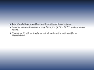
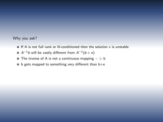
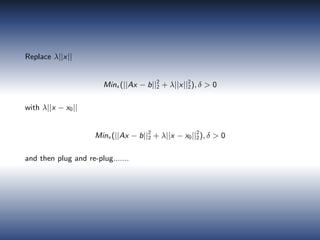
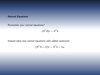
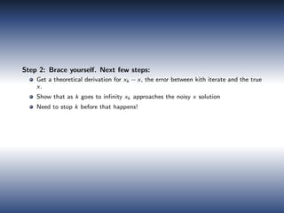
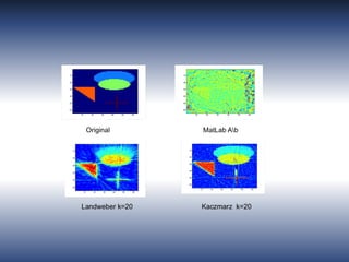
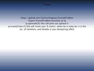
This document discusses an iterative approach to Tikhonov regularization for matrix inversion, particularly in handling ill-conditioned systems using techniques like regularization and single value decomposition (SVD). It outlines the methodology for stabilizing solutions to linear equations by adding regularization terms, comparing Tikhonov regularization to truncated SVD, and emphasizes the importance of selecting an appropriate lambda for effective results. Practical applications include image reconstruction in various fields, and it provides code references for implementing the discussed methods.

1. Iterative Approach to the Tikhanov Regularization
Problem in Matrix Inversion using Numpy
Katya Vasilaky1
November 21, 2015
1
New Yorker @ Columbia University

2. Matrix inversion problems have been around a while.

3. They’re not easy.

4. But relevant.

7. Inverse problems: compute information about some “interior” properties using
“exterior” measurements.
Tomography: Xray source − > Object − > Dampening
Inference: Attributes − > Effect Size − > Outcome
Machine Learning: Features − > Predictors − > Classifier

8. X is my back.
Problem.
Don’t know x.
Figure: Xray of Spine

9. Solution.
Throw A at x (Ax)
Collect b
Infer x (x = A−1
b).
or for linear regression....
β = (XT
X)−1
(XT
Y )

11. Methodology
The pseudoinverse solution, which always exists, is often computed as the
unique, minimum norm solution to the least-squares formulation
ˆx = Minx ||Ax − b||2
2
such that ||x||2
2 solves for the minimum.
Think of an underdetermined system of equations:
x + y + z = 1 (1)
x + y + 2z = 3 (2)
There are many solutions.
The pseudo inverse is not very useful for applications.

12. Lots of useful inverse problems are ill-conditioned linear systems.
Standard numerical methods x = A−1b or β = (XT X)−1XT Y produce useless
results.
That A (or X) will be singular or not full rank, so it’s not invertible, or
ill-conditioned

13. If you perturb b a little bit, x = A−1
(b + e)
Will map to something crazy!

14. Why you ask?
If A is not full rank or ill-conditioned then the solution x is unstable
A−1b will be vastly different from A−1(b + e)
The inverse of A is not a continuous mapping − > b
b gets mapped to something very different than b+e

15. What do people do then?
Regularization problems formulate a nearby problem, which has a more stable
solution:
Minx (||Ax − b||2
2 + λ||x||2
2), δ > 0
where we introduce the term λ||x||2
2 perturbing the least-squares formulation.
The regularization can be L1 (Lasso) or L2. Typically L2 (Tikhanov and
Truncated SVD) better. Most people try to choose a good lambda, and solve
the above, hoping that they’re close to the noiseless solution. Which penalizes
outliers more?

16. Problem with regularization is how to choose λ or how much to truncate.
Tikhonov and truncated SVD are equivalent in that chopping off singular
values is equivalent to choosing a λ?
Minx (||Ax − b||2
2 + λ||x||2
2), δ > 0
This solution: Instead of computing a solution we compute a sequence of
solutions which approximates the noiseless solution (A−
1b) on its way to the
noisy (A−
1(b + e) solution.

18. Replace λ||x||
Minx (||Ax − b||2
2 + λ||x||2
2), δ > 0
with λ||x − x0||
Minx (||Ax − b||2
2 + λ||x − x0||2
2), δ > 0
and then plug and re-plug.......

19. Normal Equations
Remember your normal equations?
(AT
A)x = AT
b
Instead solve new normal equations with added constraint:
(AT
A + λI)x = AT
b + λx0

20. Solution for x1 is:
x1 = (AT
A + λI)−1
AT
b + λ(AT
A + λI)−1
x0
and the kth iterate is:
xk = Σk
i=1λi−1
((AT
A + λI)−1
(AT
b) + λk
(AT
A + λI)−1
x0)

21. Now we the use single value decomposition (SVD) of A: A = UΣV T
,
σ1, .., σn, 0....0) ∈ Rmxn
with σ1 ≥ σ2 ≥ · · · ≥ σn > 0, where n is the rank of A,
we then obtain after a lot of derivation, the following kth
iterate.
V




1
σ1
− 1
σ1
( λ
λ+σ2
1
)k
. . . 0 . . . 0
...
...
...
0 . . . 1
σn
− 1
σn
( λ
λ+σ2
n
)k
0 . . . 0



 UT
b
For practical ease–I’m setting x0=0. It does not affect the solution.

22. Step 1
InverseProblem codes the above formula to invert A.
So inverse of A times b from InverseProblem will give us the x back.
Let’s try it out using the Inverse Problem package!
https://github.com/kathrynthegreat/InverseProblem

23. Step 2: Brace yourself. Next few steps:
Get a theoretical derivation for xk − x, the error between kith iterate and the true
x.
Show that as k goes to infinity xk approaches the noisy x solution
Need to stop k before that happens!

24. First, look at the residual error against the number of iterations.
One thing is sure. We want λ > 1

25. Next, it turns out (from experiments), that xk passes the true noiseless x when
the residual error ||Axk − b|| “turns,” a heuristic that still needs a proof.
Somehow this minimizes the error between the kith iterate and the true x:
xk − x expression.
(S1)
-V




1
σ1
( λ
λ+σ2
1
)k
. . . 0 0 . . . 0
...
...
...
0 . . . 1
σn
( λ
λ+σ2
n
)k
0 . . . 0



 UT
b
(S2) V




1
σ1
− 1
σ1
( λ
λ+σ2
1
)k
. . . 0 0 . . . 0
...
...
...
0 . . . 1
σn
− 1
σn
( λ
λ+σ2
n
)k
0 . . . 0



 UT
e

27. Now that we’ve seen the tractable cases. Here are some other uses.
We will reconstruct an image from projections. Some reconstructions from
projections are:
1 CT scans
2 MRI
3 Oil Exploration
4 Seismic imaging

31. Notes
Iterative approach is good for extremely ill conditioned matrices that are large.
For small matrices there are other approaches.
This approach is good for images because you can see when you’re doing
better-the image is clearer.
We need to see the graph (or the picture) to get an idea about lambda and k, the
good news is that we don’t have to know them optimally as in classical Tikhonov.
Otherwise if we know something about e (like it’s SD or norm ||e||) we can plot
that error graph (still need to package that)
Remember, of course, that if the data are extremely noisy then it is worthless, so
no recovery is possible.

32. Thanks.
https://github.com/kathrynthegreat/InverseProblem
import InverseProblem.functions as ip
ip.optimalk(A) this will print out optimal k
ip.invert(A,be,k,l) this will invert your A matrix, where be is noisy be, k is the
no. of iterations, and lambda is your dampening effect