Download as PDF, PPTX
![Dually flat spaces: Canonical Bregman divergences
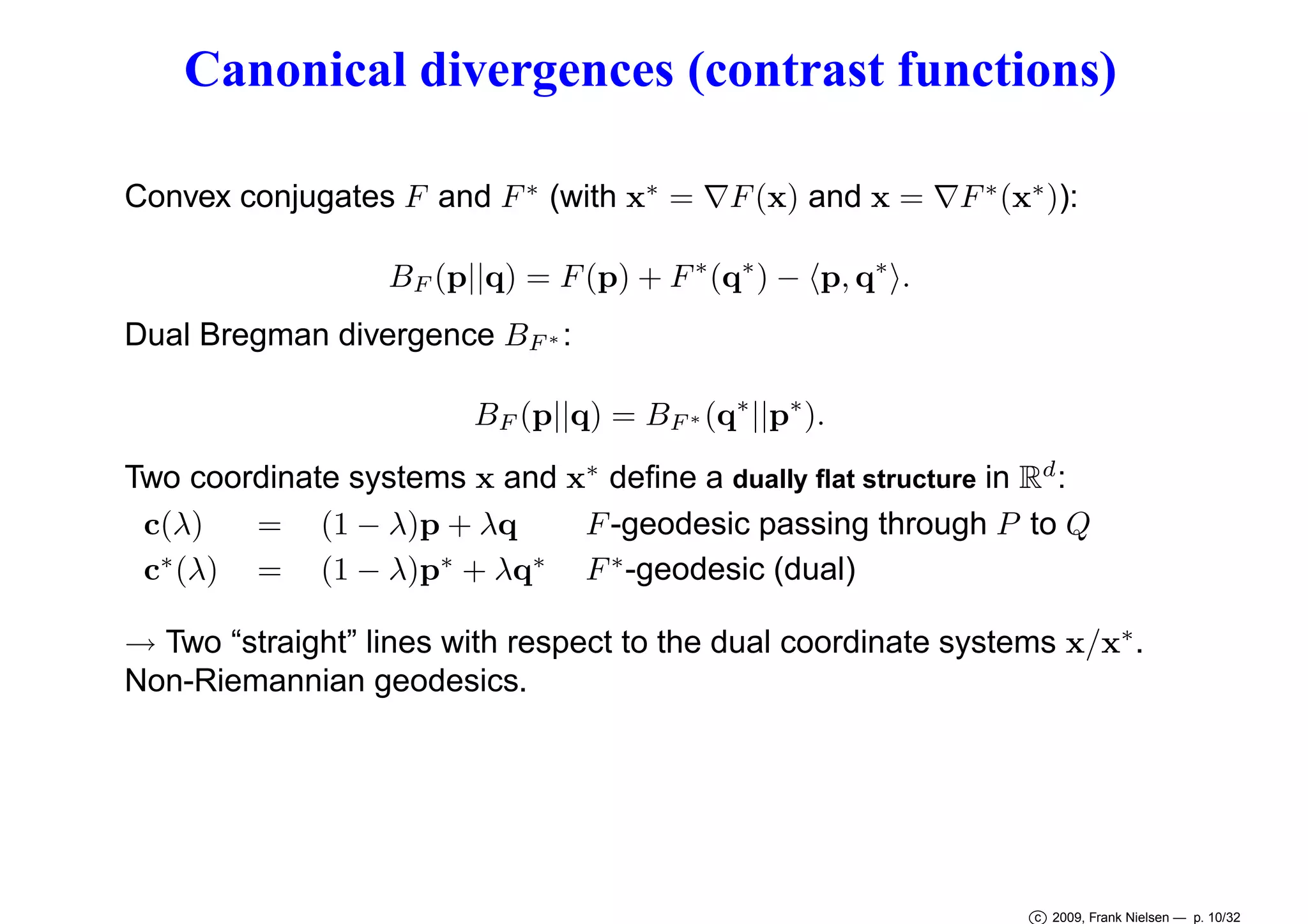
Strictly convex and differentiable generator F : Rd → R.
Bregman divergence between any two vector points p and q :
DF (p||q) = F (p) − F (q) − p − q, ∇F (q) ,
where ∇F (x) denote the gradient of F at x = [x1 ... xd ]T .
F
ˆ
p
DF (p||q)
ˆ
q
Hq
X
F (x) = xT x =
F (x) =
i pi log
d
i=1
pi
qi
d
i=1
q
p
x2 −→ squared Euclidean distance: p − q
i
2.
xi log xi (Shannon’s negative entropy) −→ Kullback-Leibler divergence:
c 2009, Frank Nielsen — p. 8/32](https://image.slidesharecdn.com/done-isvd2009-slide-131114202103-phpapp02/75/Slides-The-dual-Voronoi-diagrams-with-respect-to-representational-Bregman-divergences-ISVD-2009-8-2048.jpg)
![Representational Bregman divergences
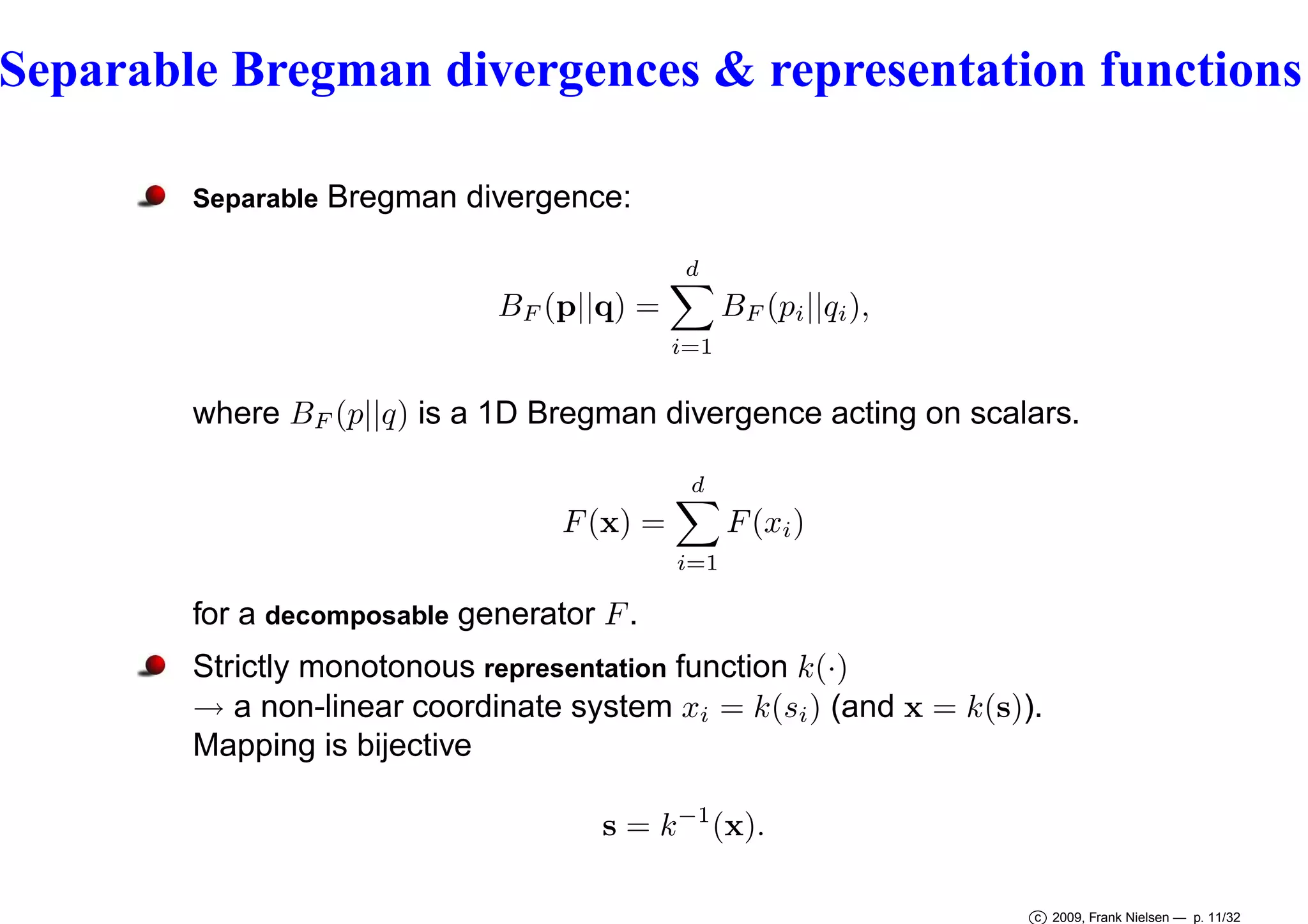
Bregman generator
d
d
U (k(si )) = F (s)
U (xi ) =
U (x) =
i=1
i=1
with F = U ◦ k.
Dual 1D generator U ∗ (x∗ ) = maxx {xx∗ − U (x)} induces dual
coordinate system x∗ = U ′ (xi ), where U ′ denotes the derivative of U .
i
′
∇U (x) = [U (x1 ) ... U ′ (xd )]T .
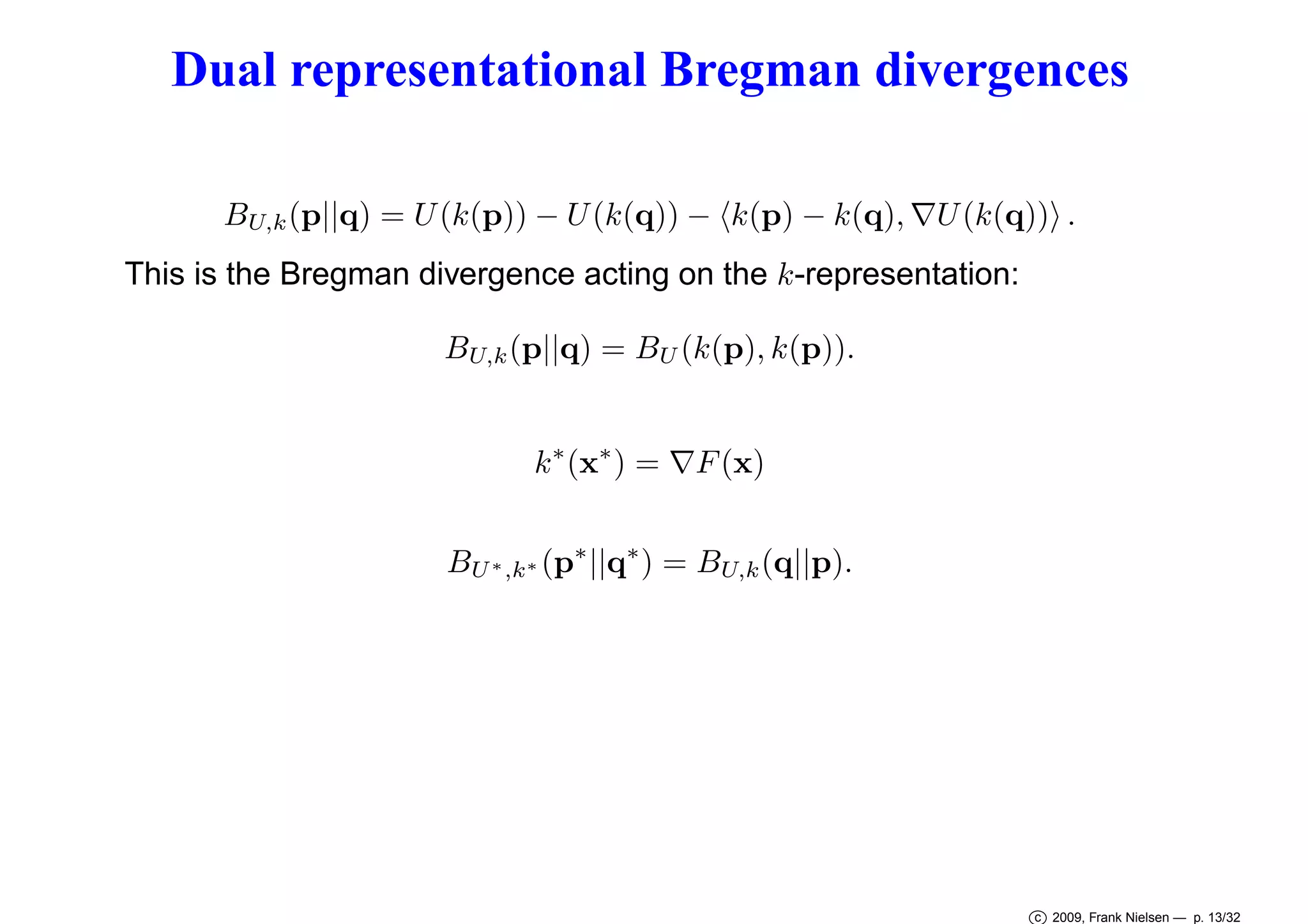
Canonical separable representational Bregman divergence:
BU,k (p||q) = U (k(p)) + U ∗ (k ∗ (q∗ )) − k(p), k ∗ (q∗ ) ,
with k ∗ (x∗ ) = U ′ (k(x)).
Often, a Bregman by setting F = U ◦ k. But although U is a strictly convex and differentiable
function and k a strictly monotonous function, F = U ◦ k may not be strictly convex.
c 2009, Frank Nielsen — p. 12/32](https://image.slidesharecdn.com/done-isvd2009-slide-131114202103-phpapp02/75/Slides-The-dual-Voronoi-diagrams-with-respect-to-representational-Bregman-divergences-ISVD-2009-12-2048.jpg)
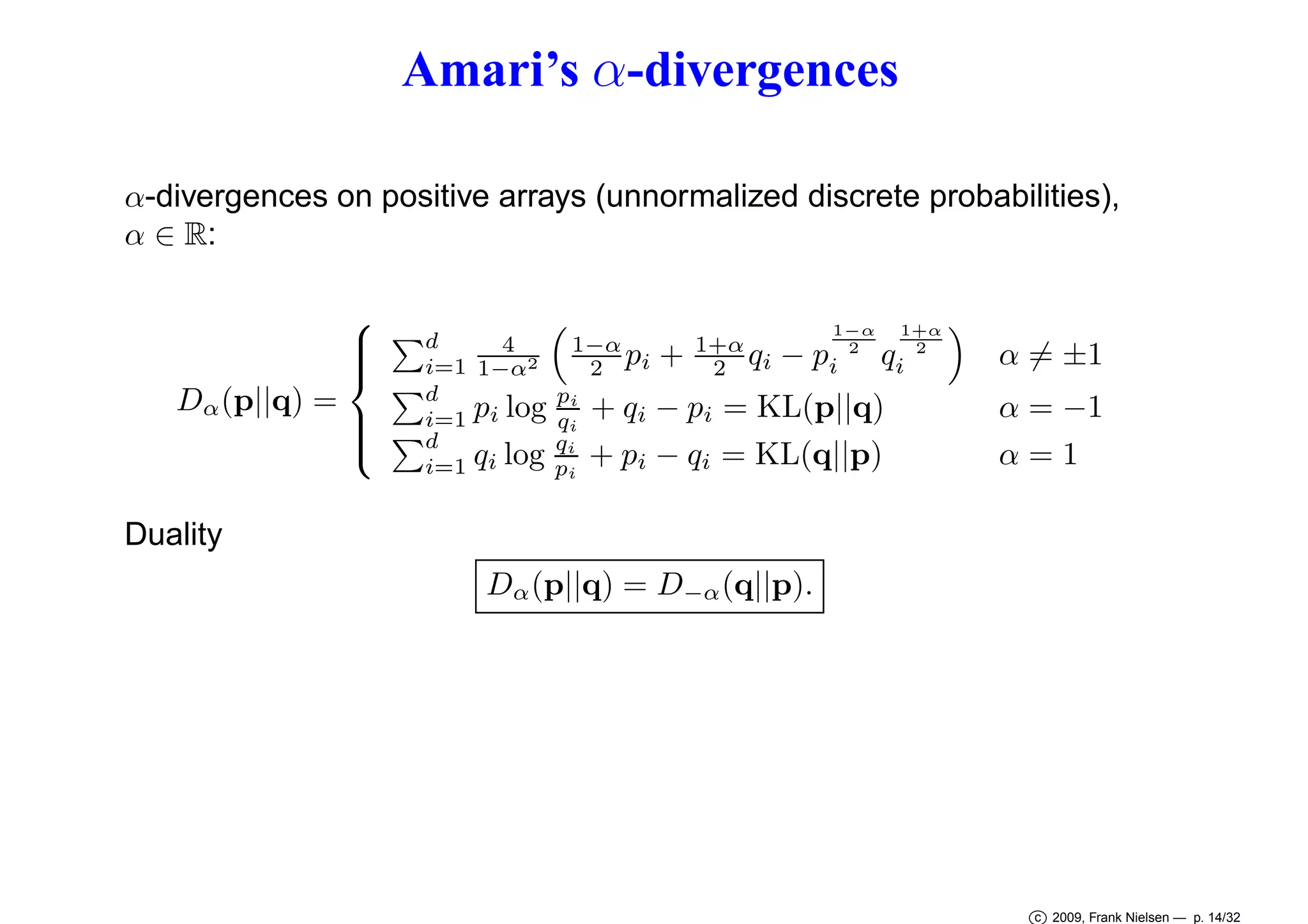
![α-divergences: Special cases of Csiszár f -divergences
Special case of Csiszár f -divergences associated with any convex
function f satisfying f (1) = f ′ (1) = 0:
d
pi f
Cf (p||q) =
i=1
qi
pi
.
For statistical measures, Cf (p||q) = EP [f (Q/P )], function of the ’likelihood
ratio’.
For α = 0, take
fα (x) =
4
1 − α2
1+α
1−α 1+α
+
x−x 2
2
2
Dα (p||q) = Cfα (p||q)
α-divergences are canonical divergences of constant-curvature
geometries.
α-divergences are representational Bregman divergences in disguise.
c 2009, Frank Nielsen — p. 15/32](https://image.slidesharecdn.com/done-isvd2009-slide-131114202103-phpapp02/75/Slides-The-dual-Voronoi-diagrams-with-respect-to-representational-Bregman-divergences-ISVD-2009-15-2048.jpg)
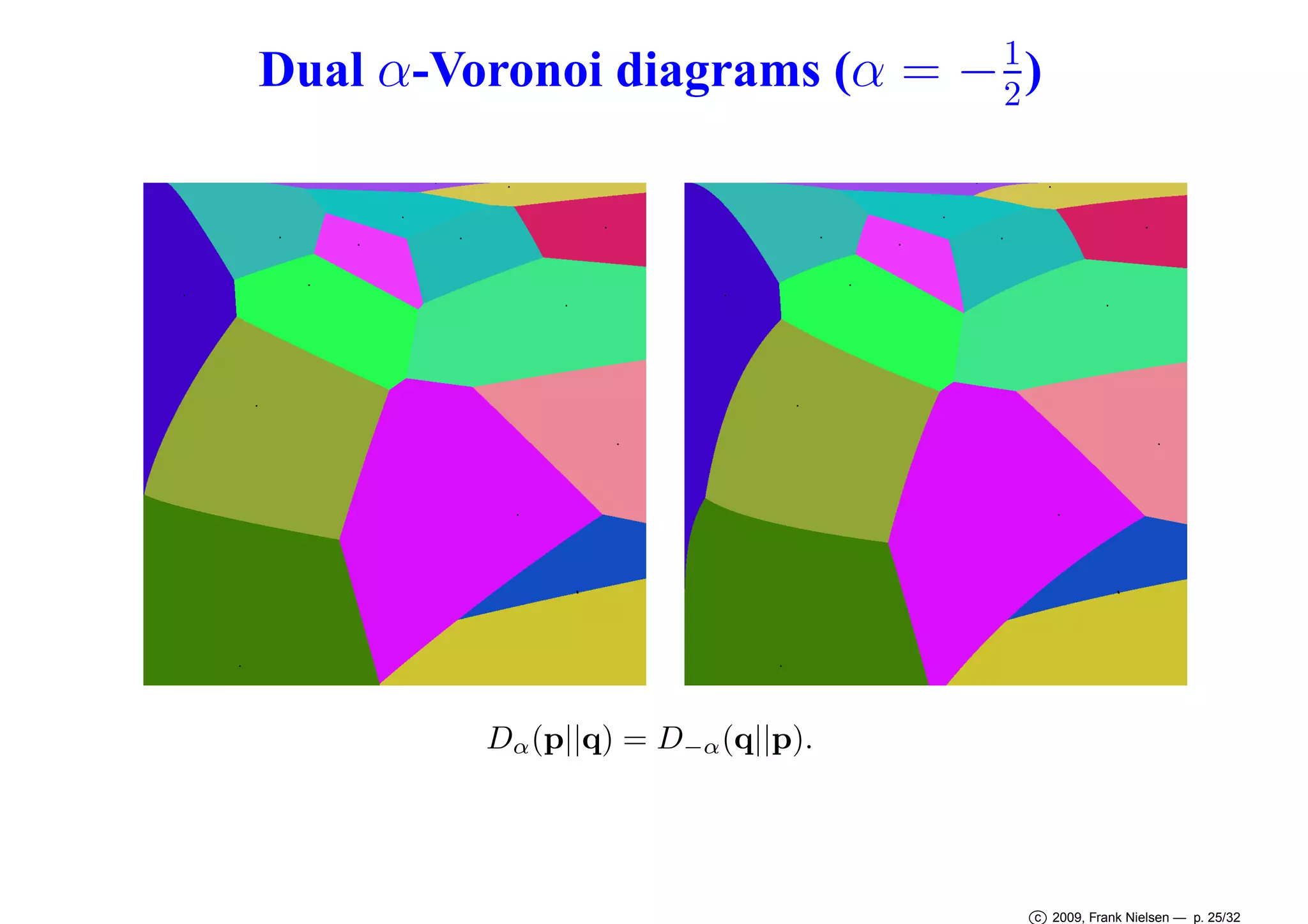
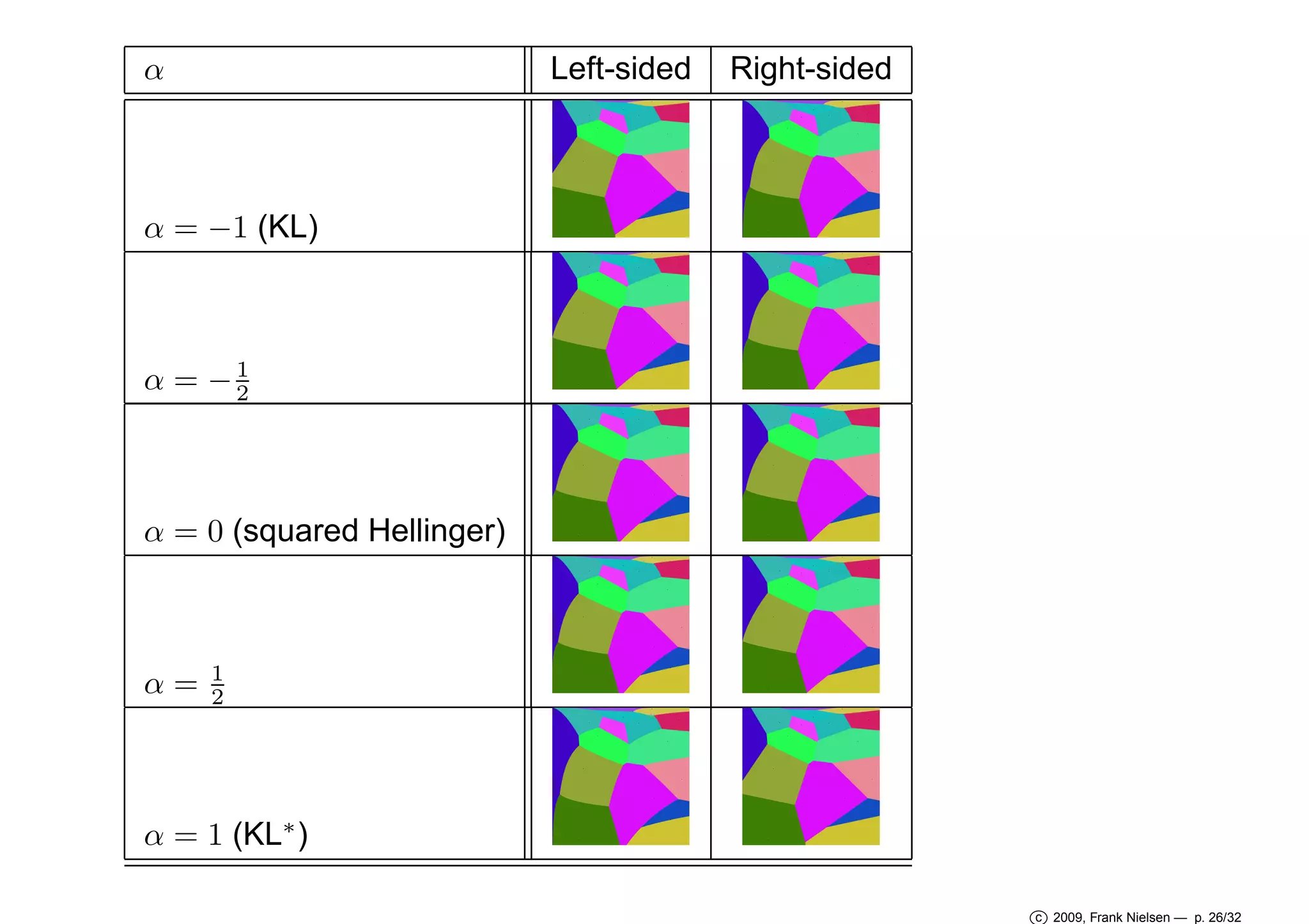
![α-Voronoi diagrams
Right-sided α-bisectors
Hα (p, q) : {x ∈ X |Dα (p|| x ) = Dα (q|| x )}
for α = ±1.
=⇒ Hα (p, q) :
i
1+α
2
Letting X = [x1
1+α
2
... xd
1−α
1−α
1+α
1−α
2 (q 2
− p 2 ) = 0.
(pi − qi ) + x
2
]T , we get hyperplane bisectors:
Xi (q
Hα (p, q) :
i
1−α
2
−p
1−α
2
)+
i
1−α
(pi − qi ) = 0.
2
Right-sided α-Voronoi diagram is affine in the k(x) = x
d
with complexity O(n⌈ 2 ⌉ ).
1+α
2
-representation
Indeed, D(X||Pi ) = BU,k (x||pi ) ≤ D(X||Pj ) = BU,k (x||pj ) ⇐⇒ BU (k(x)||k(pi )) ≤
BU (k(x)||k(pj )).
c 2009, Frank Nielsen — p. 24/32](https://image.slidesharecdn.com/done-isvd2009-slide-131114202103-phpapp02/75/Slides-The-dual-Voronoi-diagrams-with-respect-to-representational-Bregman-divergences-ISVD-2009-24-2048.jpg)
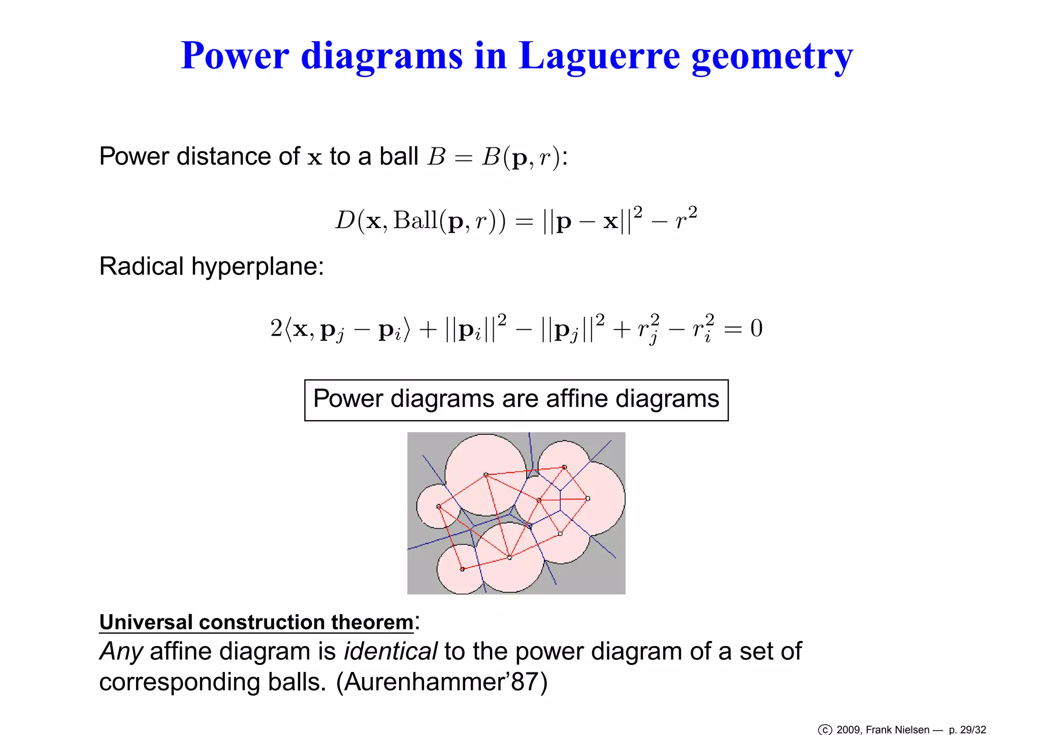
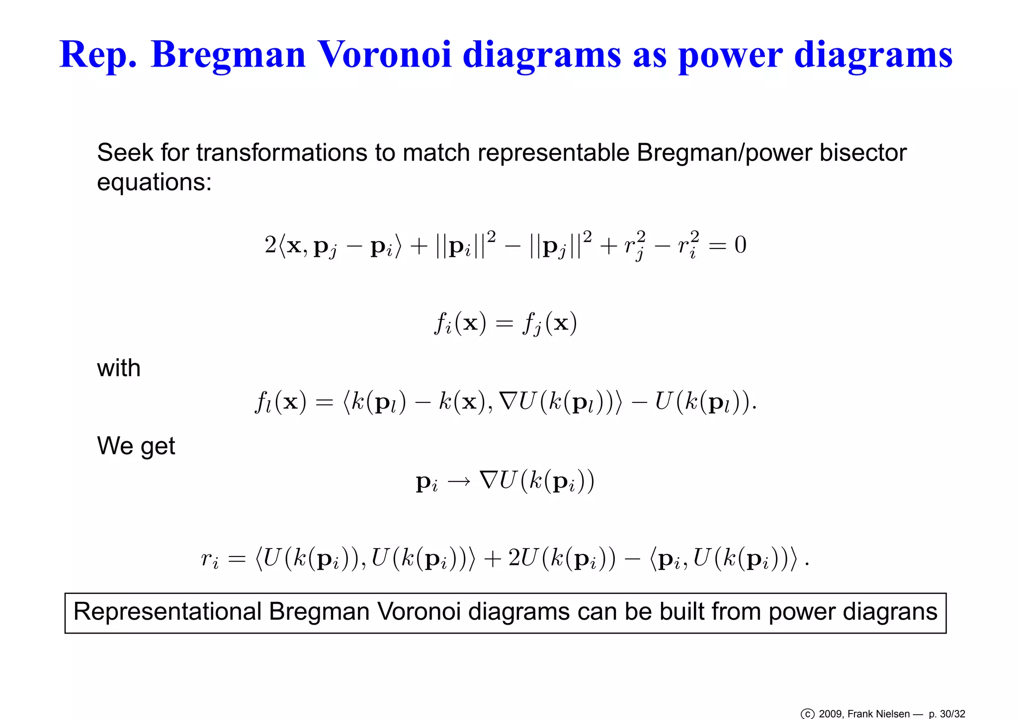
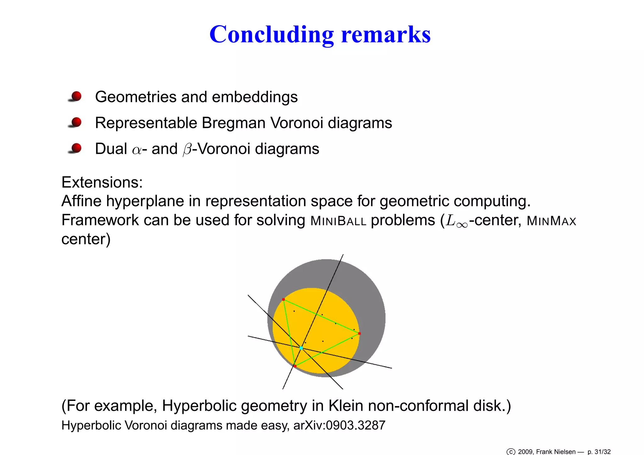

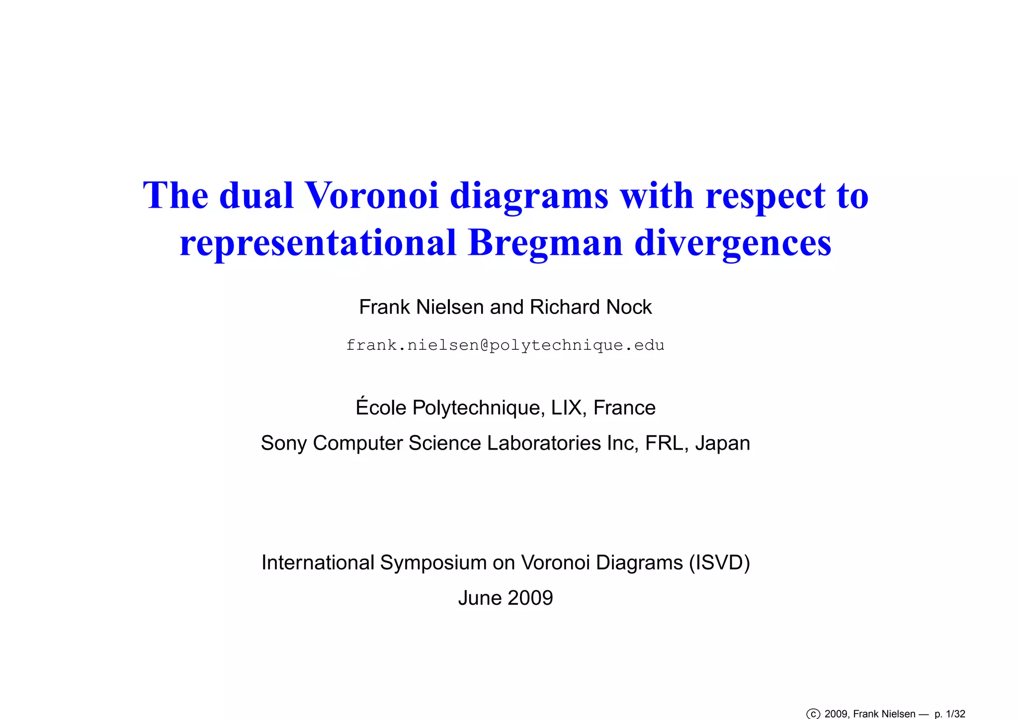
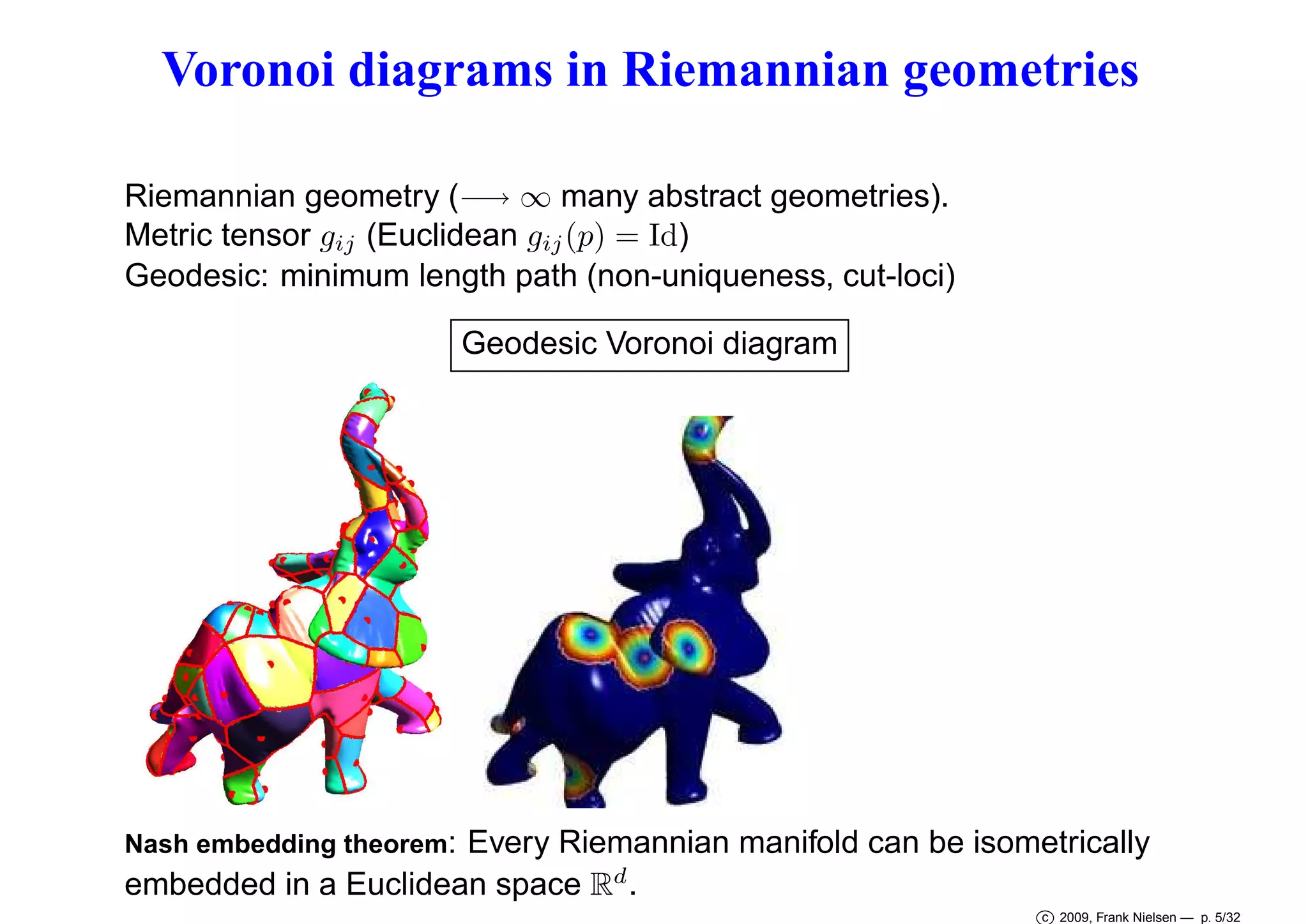
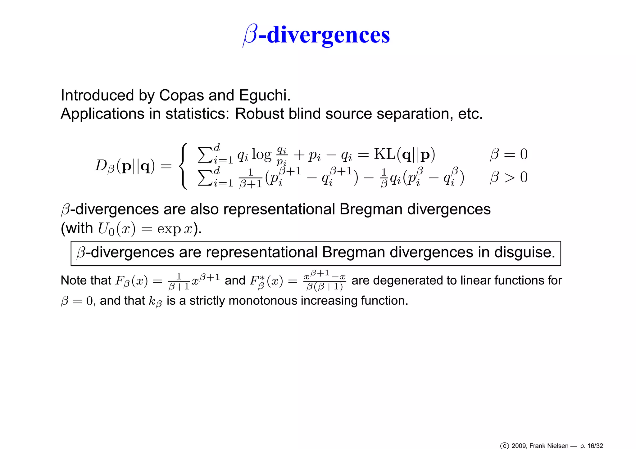
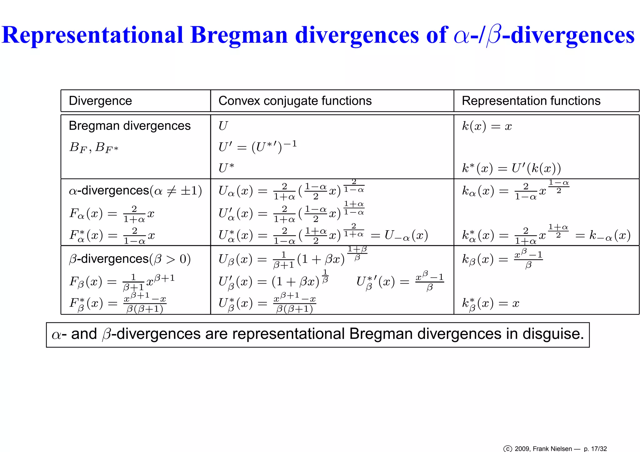
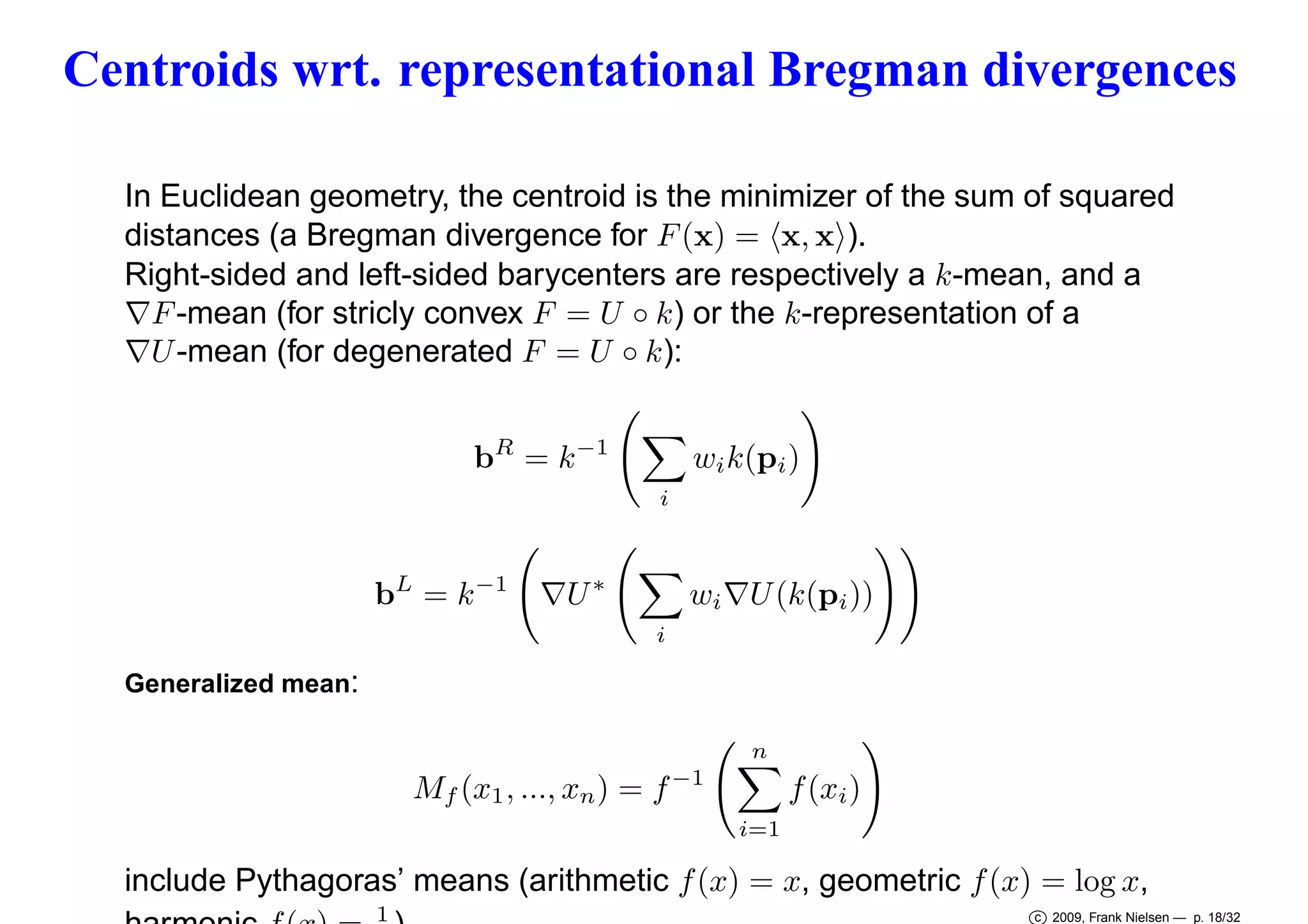
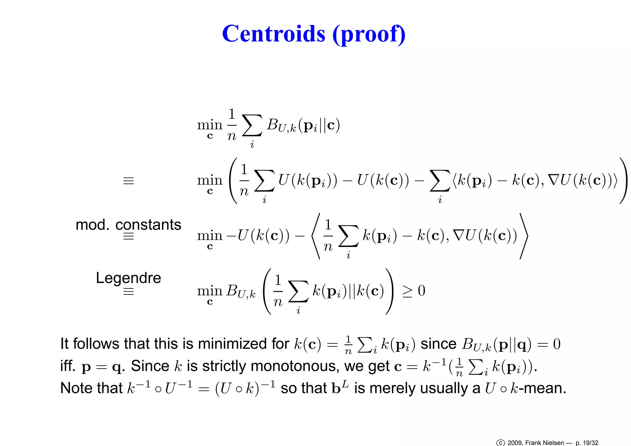
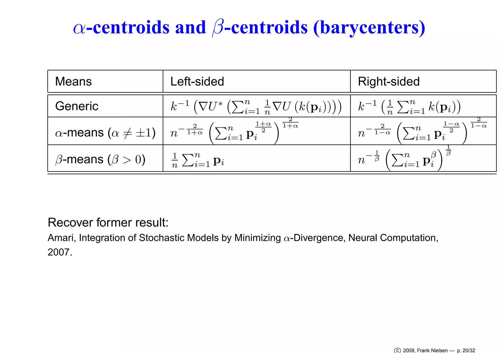
This document discusses Voronoi diagrams in various geometries beyond Euclidean space. It begins by introducing ordinary Voronoi diagrams based on Euclidean distance. It then discusses Voronoi diagrams in non-Euclidean geometries like spherical and hyperbolic spaces. It also discusses Voronoi diagrams in Riemannian geometries defined by a metric tensor, as well as information geometries based on probability distributions. The document introduces Bregman divergences and shows how Voronoi diagrams can be defined using these divergences in dually flat spaces. It specifically discusses α-divergences and β-divergences as examples of representational Bregman divergences. It concludes by discussing centroids


![Inference in generative models using the Wasserstein distance [[INI]](https://cdn.slidesharecdn.com/ss_thumbnails/inewton-170706120746-thumbnail.jpg?width=640&height=640&fit=bounds)


![Coded Agents – with UiPath SDK + LangGraph [Virtual Hands-on Workshop]](https://cdn.slidesharecdn.com/ss_thumbnails/codedagentsdeck-251215155422-5497c599-thumbnail.jpg?width=640&height=640&fit=bounds)


