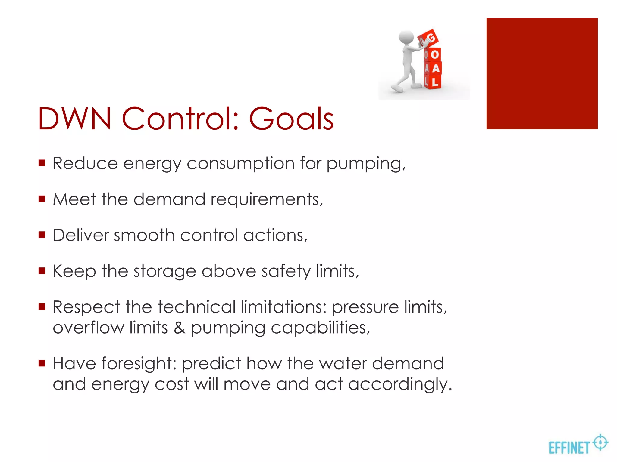
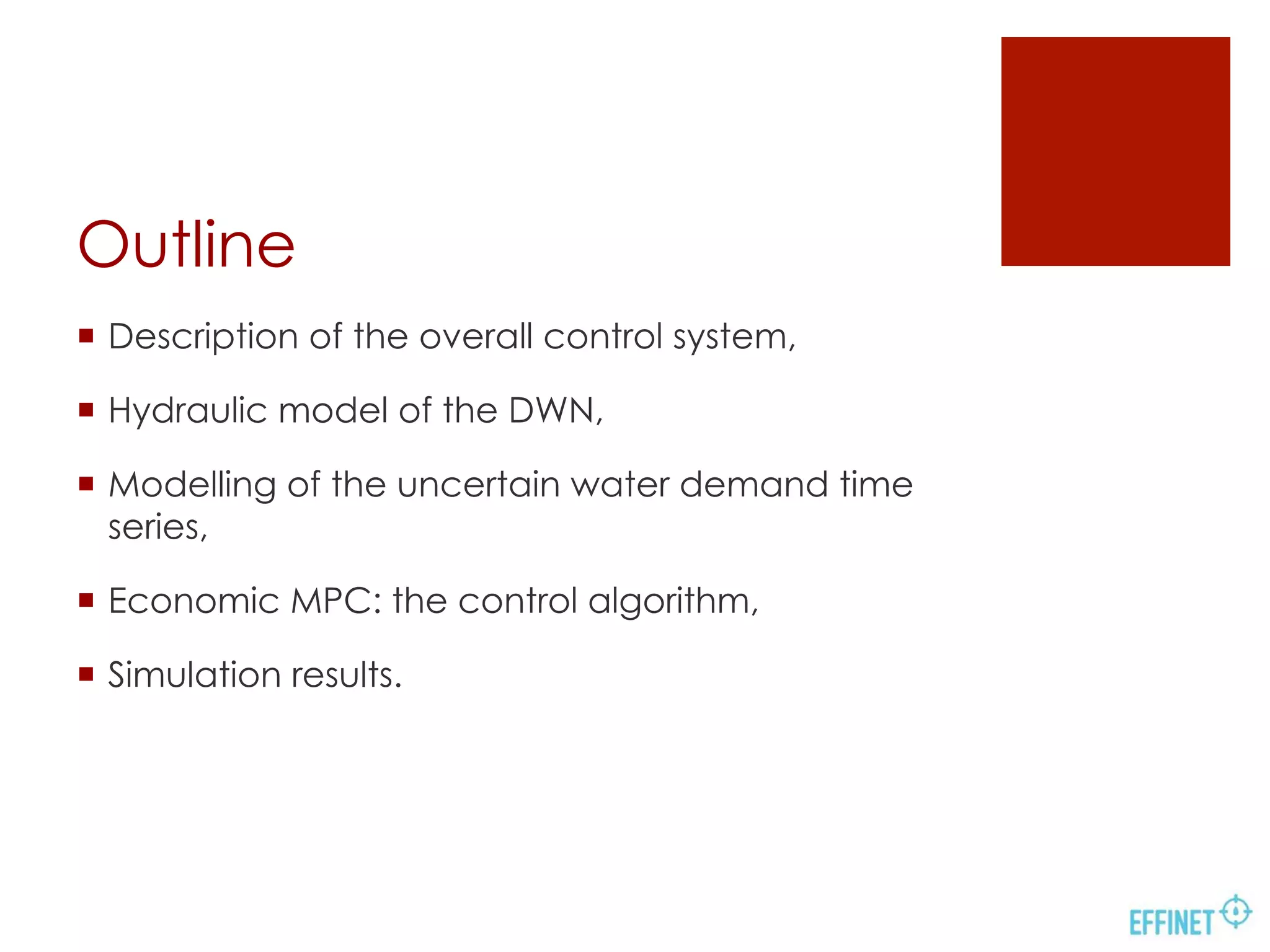
Download as PDF, PPTX
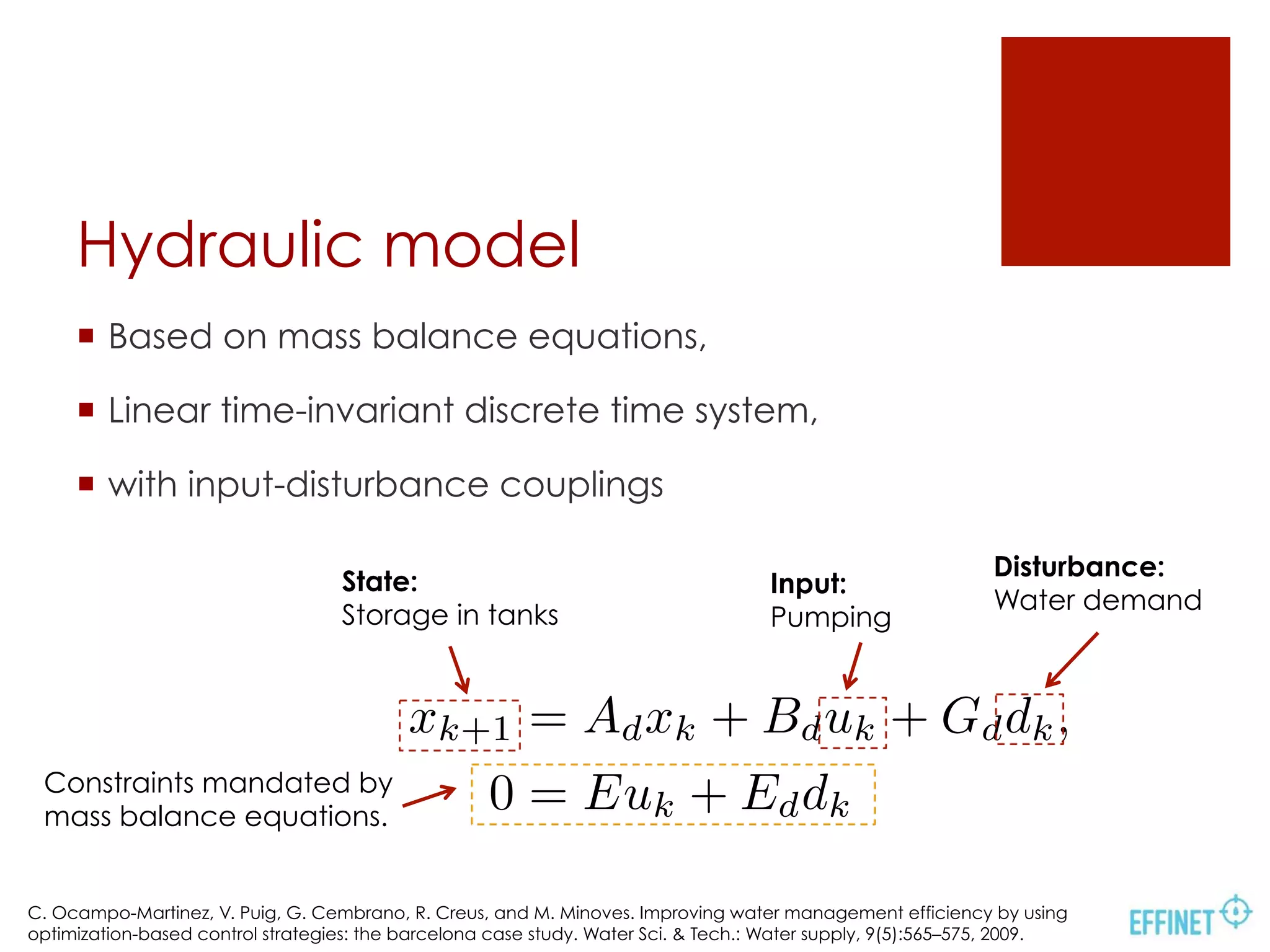
![Water demand forecasting
RBF-SVM model
¡ PMSE24 = 0.0065,
¡ 229 parameters (complex),
¡ 10-fold cross-validation
gave q2 = 0.9952,
¡ Explanatory variables:
200 past demands plus a
set of binary calendar
variables,
¡ Stringent confidence
intervals.
3250 3260 3270 3280 3290 3300 3310 3320
3
4
5
6
7
8
9
10
x 10
−3
Time [hr]
Demand[m
3
hr
−1
]
RBF−SVM Prediction](https://image.slidesharecdn.com/effinetifacpresentation-140819051639-phpapp01/75/Water-demand-forecasting-for-the-optimal-operation-of-large-scale-water-networks-8-2048.jpg)
![0 20 40 60 80 100 120 140 160 180 200
0
0.01
0.02
0.03
0.04
0.05
0.06
0.07
Time [h]
WaterDemandFlow[m3
/h]
Forecasting of Water Demand
FuturePast
Water demand forecasting
BATS model
¡ Box-Cox transformation,
ARMA errors, Trends and
Seasonality,
¡ PMSE24 = 0.0043,
¡ with just 26 parameters,
¡ Very stringent confidence
intervals.](https://image.slidesharecdn.com/effinetifacpresentation-140819051639-phpapp01/75/Water-demand-forecasting-for-the-optimal-operation-of-large-scale-water-networks-9-2048.jpg)
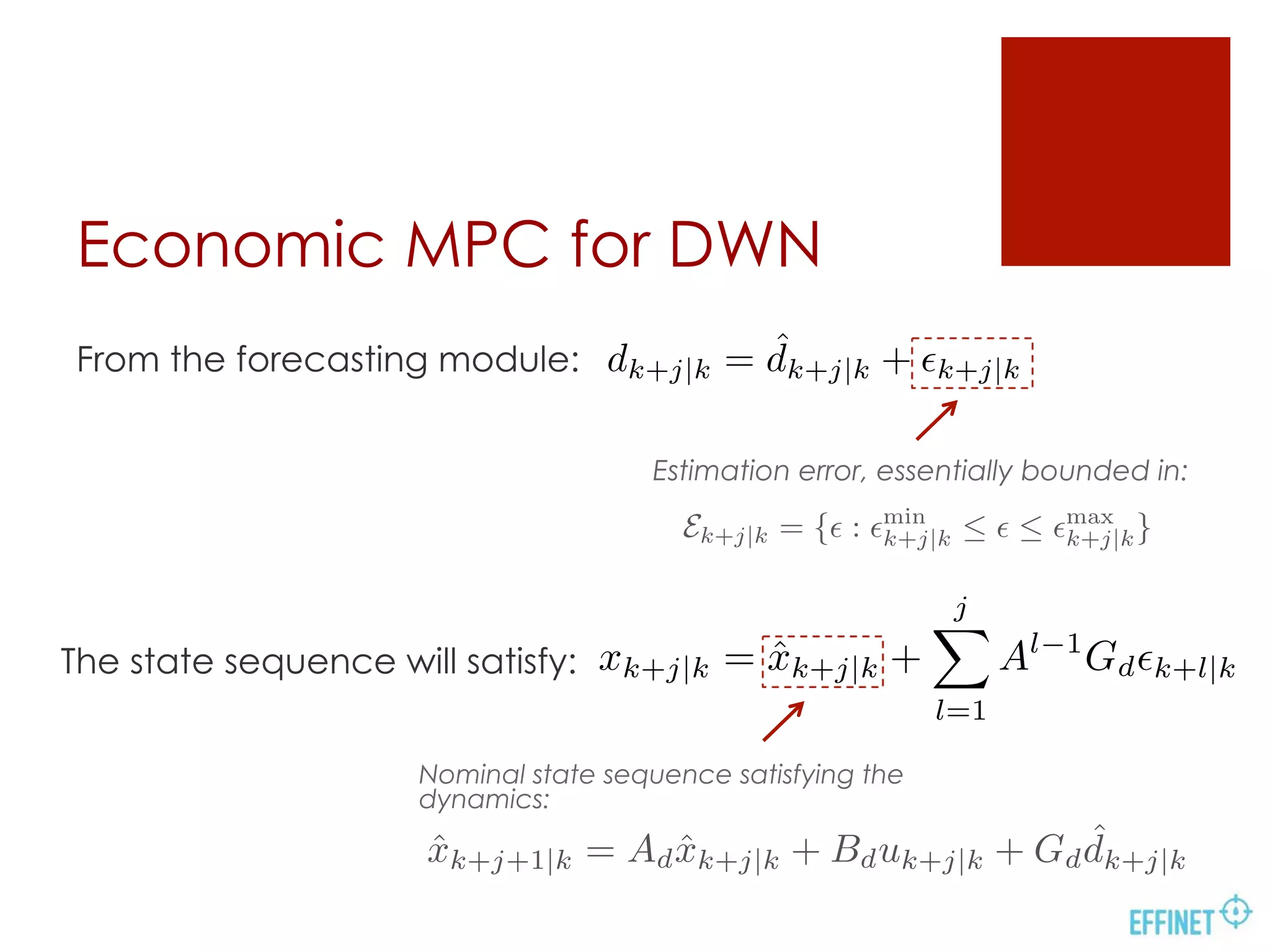
![Economic MPC for DWN
4500 4505 4510 4515 4520 4525 4530 4535 4540 4545
0.2
0.4
0.6
0.8
1
1.2
1.4
1.6
1.8
x 10
4
Time [hr]
Volume[m3
]
Safety Volume
Minimum Volume
Maximum Volume
MPC Upper Bound
MPC Lower Bound
Predicted Trajectory
Closed−loop trajectory
ˆxk+j|k 2 X
iM
j=1
Aj 1
GdEk+j|k
Bounds on the predicted state
sequence calculated by:
The sparsity of Gd enables this
computation!](https://image.slidesharecdn.com/effinetifacpresentation-140819051639-phpapp01/75/Water-demand-forecasting-for-the-optimal-operation-of-large-scale-water-networks-13-2048.jpg)
![Economic MPC for DWN
4500 4505 4510 4515 4520 4525 4530 4535 4540 4545
0.2
0.4
0.6
0.8
1
1.2
1.4
1.6
1.8
x 10
4
Time [hr]
Volume[m3
]
Safety Volume
Minimum Volume
Maximum Volume
MPC Upper Bound
MPC Lower Bound
Predicted Trajectory
Closed−loop trajectory
ˆxk+j+1|k = Ad ˆxk+j|k + Bduk+j|k+
+ Gd
ˆdk+j|k
Predicted state sequence
according to:](https://image.slidesharecdn.com/effinetifacpresentation-140819051639-phpapp01/75/Water-demand-forecasting-for-the-optimal-operation-of-large-scale-water-networks-14-2048.jpg)
![MPC: Performance
10 20 30 40 50 60 70 80 90
0.2
0.4
0.6
0.8
MPC Control Action (1~20)
ControlAction
10 20 30 40 50 60 70 80 90
0.2
0.4
0.6
0.8
MPC Control Action (21~46)
ControlAction
10 20 30 40 50 60 70 80 90
0
0.1
0.2
Time [hr]
WaterCost[e.u.]
MPC in action
• 88 demand nodes
• 63 tanks
• 114 pumping stations
• 17 flow nodes
50 100 150 200 250 300 350 400 450 500
4
5
6
7
8
Economic Cost (E.U.)
50 100 150 200 250 300 350 400 450 500
0.5
1
1.5
2
Smooth Operation Cost
0 50 100 150 200 250 300 350 400 450 500
0
2
4
6
Safety Storage Cost (× 107
)
Low price à Pumping
The system operator has
information about the
current and the
predicted operation cost.](https://image.slidesharecdn.com/effinetifacpresentation-140819051639-phpapp01/75/Water-demand-forecasting-for-the-optimal-operation-of-large-scale-water-networks-15-2048.jpg)
![5 10 15 20 25 30 35 40 45 50 55
0
20
40
60
80
100
Closed−loop MPC Simulation
Time [hr]
Repletion[%]
5 10 15 20 25 30 35 40 45 50 55
0
0.5
1
1.5
Time [hr]
Demand[m
3
/s]
MPC: Performance
10 20 30 40 50 60 70 80 90
0.2
0.4
0.6
0.8
MPC Control Action (1~20)
ControlAction
10 20 30 40 50 60 70 80 90
0.2
0.4
0.6
0.8
MPC Control Action (21~46)
ControlAction
10 20 30 40 50 60 70 80 90
0
0.1
0.2
Time [hr]
WaterCost[e.u.]
Foresight: Tanks starts
loading up before a
DMA asks for water.](https://image.slidesharecdn.com/effinetifacpresentation-140819051639-phpapp01/75/Water-demand-forecasting-for-the-optimal-operation-of-large-scale-water-networks-16-2048.jpg)


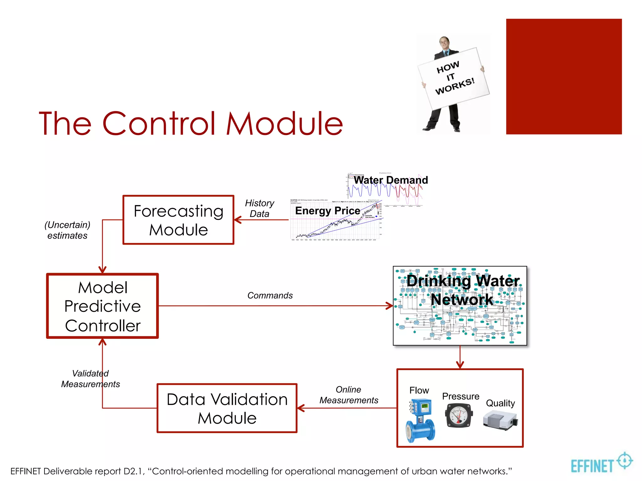
This document summarizes research on using model predictive control (MPC) for optimizing the operation of large-scale drinking water networks. Key points: - MPC aims to reduce energy costs while meeting demand and respecting constraints, using forecasts of water demand and energy prices. - Demand is forecasted using SARIMA, BATS and RBF-SVM models, with RBF-SVM achieving the best accuracy. - A hydraulic model is developed to predict network state based on inputs, disturbances, and constraints. - MPC optimizes pumping over a horizon while respecting constraints, using demand forecasts to anticipate future needs. - Simulation results on a real network show MPC achieving low costs while


