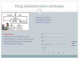
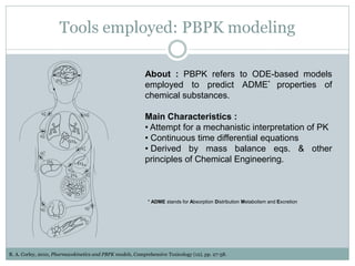
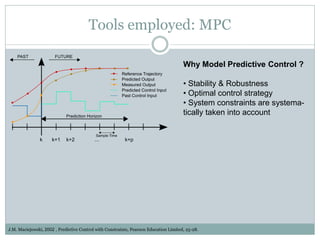
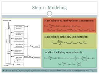
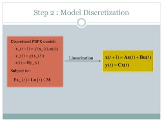
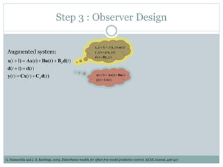
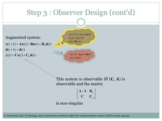
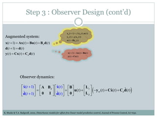
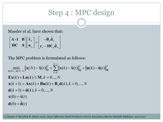
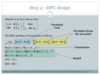
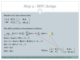
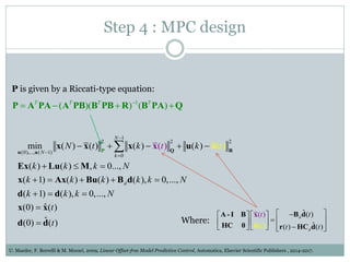
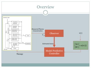
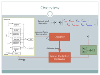
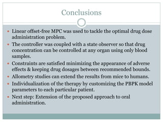
This document describes a physiologically based pharmacokinetic (PBPK) modeling and model predictive control (MPC) approach for optimal drug administration. It involves 4 main steps: 1) Developing PBPK models using mass balance equations to describe drug distribution in compartments like plasma, red blood cells, and kidneys. 2) Discretizing the PBPK models and designing an observer to estimate unmeasured states using the measured plasma concentration. 3) Formulating an MPC problem to determine optimal drug administration inputs over a prediction horizon while satisfying constraints like toxicity limits. 4) Solving the MPC problem online to determine the optimal control action and adjust the drug dosage based on the

1. Physiologically Based
Pharmacokinetic Modeling and
Predictive Control
An integrated approach for optimal drug administration
P. Sopasakis, P. Patrinos, S. Giannikou, H.
Sarimveis.
Presented in the 21 European Symposium on
Computer-Aided Process Engineering

2. Drug administration strategies
Open loop drug
administration based on
average population
pharmacokinetic studies
Evaluation: Toxicity Alert!
• No feedback
• Suboptimal drug administration
• The therapy is not individualized
• High probability for side effects!
W. E. Stumpf, 2006, The dose makes the medicine, Drug Disc. Today, 11 (11,12), 550-555

3. Drug administration strategies
Patients for which
the therapy works
beneficially
Patients prone to
side-effects

4. Drug administration strategies
The treating doctor
examines the patient
regularly and readjusts the
dosage if necessary
Evaluation :
• A step towards therapy individualization
• Again suboptimal
• Again there is a possibility for side effects
• Empirical approach

5. Drug administration strategies
Computed-Aided
scheduling of drug
administration
Evaluation:
• Optimal drug administration
• Constraints are taken into account
• Systematic/Integrated approach
• Individualized therapy

6. What renders the problem so interesting?
 Input (administered dose) & State (tissue conce-
ntration) constraints (toxicity).
 Only plasma concentration is available (need to
design observer).
 The set-point value might be different among patients
and might not be constant.

7. Problem Formulation
Problem: Control the concentration of DMA in the
kidneys of mice (set point: 0.5μg/lt) while the i.v. influx
rate does not exceed 0.2μg/hr and the concentration in the
liver does not exceed 1.4μg/lt.

8. Tools employed: PBPK modeling
About : PBPK refers to ODE-based models
employed to predict ADME* properties of
chemical substances.
Main Characteristics :
• Attempt for a mechanistic interpretation of PK
• Continuous time differential equations
• Derived by mass balance eqs. & other
principles of Chemical Engineering.
* ADME stands for Absorption Distribution Metabolism and Excretion
R. A. Corley, 2010, Pharmacokinetics and PBPK models, Comprehensive Toxicology (12), pp. 27-58.

9. Tools employed: MPC
Why Model Predictive Control ?
• Stability & Robustness
• Optimal control strategy
• System constraints are systema-
tically taken into account
J.M. Maciejowski, 2002 , Predictive Control with Constraints, Pearson Education Limited, 25-28.

10. Step 1 : Modeling
Mass balance eq. in the plasma compartment:
dC plasma
Vplasma  QskinCv , skin  Qlung Cv ,lung  Qkidney Cv ,kidney 
dt
Qblood Cv ,blood  Qresidual Cv ,residual  u  ( RBC CRBC   plasma C plasma )  QC C plasma
Mass balance in the RBC compartment:
dCRBC
Vplasma   plasmaC plasma   RBC CRBC
dt
And for the kidney compartments :
 
 Qkidney  C Arterial  Cv ,kidney    kidney  Cv ,kidney 
dCkidney Ckidney
Vkidney
   kkidney Akidney

dt  Pkidney 
dCv ,kidney  Ckidney 
Vkidney   kidney  Cv ,kidney  
dt  Pkidney 
 
M. V. Evans et al, 2008, A physiologically based pharmacokin. model for i.v. and ingested DMA in mice, Toxicol. sci., Oxford University Press, 1 – 4 .

11. Step 2 : Model Discretization
Discretized PBPK model:
x m (t  1)  f (x m (t ), u(t ))
y m (t )  g (x m (t )) x(t  1)  Ax(t )  Bu(t )
Linearization
z (t )  Hy m (t )
y (t )  Cx(t )
Subject to :
Exm  t   Lu  t   M

12. Step 3 : Observer Design
x m (t  1)  f (x m (t ), u(t ))
Augmented system: y m (t )  g (x m (t ))
z (t )  Hy m (t )
x(t  1)  Ax(t )  Bu(t )  B d d(t )
d(t  1)  d(t )
y (t )  Cx(t )  Cd d(t ) x(t  1)  Ax(t )  Bu(t )
y (t )  Cx(t )
G. Pannocchia and J. B. Rawlings, 2003, Disturbance models for offset-free model predictive control, AlChE Journal, 426-437.

13. Step 3 : Observer Design (cont’d)
x m (t  1)  f (x m (t ), u(t ))
Augmented system: y m (t )  g (x m (t ))
z (t )  Hy m (t )
x(t  1)  Ax(t )  Bu(t )  B d d(t )
d(t  1)  d(t )
y (t )  Cx(t )  Cd d(t ) x(t  1)  Ax(t )  Bu(t )
y (t )  Cx(t )
This system is observable iff (C, A) is
observable and the matrix
 A  I Bd 
 C Cd 
 
is non-singular
G. Pannocchia and J. B. Rawlings, 2003, Disturbance models for offset-free model predictive control, AlChE Journal, 426-437.

14. Step 3 : Observer Design (cont’d)
x m (t  1)  f (x m (t ), u(t ))
Augmented system: y m (t )  g (x m (t ))
z (t )  Hy m (t )
x(t  1)  Ax(t )  Bu(t )  B d d(t )
d(t  1)  d(t )
y (t )  Cx(t )  Cd d(t ) x(t  1)  Ax(t )  Bu(t )
y (t )  Cx(t )
Observer dynamics:
 x(t  1)   A Bd   x(t )  B 
ˆ ˆ L 
ˆ    ˆ  0
ˆ
   u(t )   x  y m (t )  Cx(t )  Cd d(t )
ˆ  
d(t  1)   0 I  d(t )    L d 
K. Muske & T.A. Badgwell, 2002, Disturbance models for offset-free linear model predictive control, Journal of Process Control, 617-632.

15. Step 4 : MPC design
Maeder et al. have shown that:
ˆ
 A - I B   x    B d d  
ˆ
 HC 0  u    
ˆ 
     r  HCd d 

The MPC problem is formulated as follows:
N 1
x( N )  x (t ) P   x(k )  x (t )  u(k )  u(t )
2 2 2
min Q R
u (0),...,u ( N 1)
k 0
Ex(k )  Lu(k )  M, k  0..., N
x(k  1)  Ax(k )  Bu(k )  B d d(k ), k  0,..., N
d(k  1)  d(k ), k  0,..., N
x(0)  x(t )
ˆ
ˆ
d(0)  d(t )
U. Maeder, F. Borrelli & M. Morari, 2009, Linear Offset-free Model Predictive Control, Automatica, Elsevier Scientific Publishers , 2214-2217.

16. Step 4 : MPC design
Maeder et al. have shown that:
ˆ
 A - I B   x    B d d  
ˆ Terminal
 HC 0  u    
ˆ  Cost
     r  HCd d 

Deviation from
the set-point
The MPC problem is formulated as follows:
N 1
x( N )  x (t ) P   x(k )  x (t )  u(k )  u(t )
2 2 2
min Q R
u (0),...,u ( N 1)
k 0
Ex(k )  Lu(k )  M, k  0..., N Constraints
x(k  1)  Ax(k )  Bu(k )  B d d(k ), k  0,..., N
d(k  1)  d(k ), k  0,..., N
x(0)  x(t )
ˆ Model
ˆ
d(0)  d(t )
U. Maeder, F. Borrelli & M. Morari, 2009, Linear Offset-free Model Predictive Control, Automatica, Elsevier Scientific Publishers , 2214-2217.

17. Step 4 : MPC design
Maeder et al. have shown that:
ˆ
 A - I B   x    B d d  
ˆ
 HC 0  u    
ˆ 
     r  HCd d 

The MPC problem is formulated as follows:
N 1
x( N )  x (t ) P   x(k )  x (t )  u(k )  u(t )
2 2 2
min Q R
u (0),...,u ( N 1)
k 0
Ex(k )  Lu(k )  M, k  0..., N
x(k  1)  Ax(k )  Bu(k )  B d d(k ), k  0,..., N
d(k  1)  d(k ), k  0,..., N
x(0)  x(t )
ˆ
ˆ
 A - I B   x(t )   B d d(t ) 
ˆ
d(0)  d(t ) Where:  HC 0  u(t )    
ˆ (t ) 
   r (t )  HCd d 

U. Maeder, F. Borrelli & M. Morari, 2009, Linear Offset-free Model Predictive Control, Automatica, Elsevier Scientific Publishers , 2214-2217.

18. Step 4 : MPC design
P is given by a Riccati-type equation:
P  AT PA  (AT PB)(BT PB  R)1 (BT PA)  Q
N 1
x( N )  x (t ) P   x(k )  x (t )  u(k )  u(t )
2 2 2
min Q R
u (0),...,u ( N 1)
k 0
Ex(k )  Lu(k )  M, k  0..., N
x(k  1)  Ax(k )  Bu(k )  B d d(k ), k  0,..., N
d(k  1)  d(k ), k  0,..., N
x(0)  x(t )
ˆ
ˆ
 A - I B   x(t )   B d d(t ) 
ˆ
d(0)  d(t ) Where:  HC 0  u(t )    
ˆ (t ) 
   r (t )  HCd d 

U. Maeder, F. Borrelli & M. Morari, 2009, Linear Offset-free Model Predictive Control, Automatica, Elsevier Scientific Publishers , 2214-2217.

19. Overview
Measured Plasma
Concentration
Observer r t 
C pl
Estimated states  x(t ) 
u(t )     r  t  
 
Model Predictive
Therapy Controller

20. Overview
Reconstructed Cˆ ˆ ˆ ˆ
Clung / bl Cskin Cskin / bl 
ˆ d    lung
x  C 
ˆ ˆ 
state vector :   ˆ ˆ ˆ ˆ 
 dlung dlung / blood d skin d skin / blood 
Measured Plasma
Concentration
Observer r t 
C pl
Estimated states  x(t ) 
u(t )     r  t  
 
Model Predictive
Therapy Controller

21. Results: Assumptions
Assumptions: Intravenous administration of DMA to
mice with constant infusion rate (0.012lt/hr). Prediction
Horizon was fixed to N=10 and the set point was set to
0.5μg/lt in the kidney.
Additional Restrictions: The i.v. rate does not exceed
0.2μg/hr and the concentration in the liver remains below
1.4 μg/lt.
M. V. Evans et al, 2008, A physiologically based pharmacokin. model for i.v. and ingested DMA in mice, Toxicol. sci., Oxford University Press, 1 – 4 .

22. Results: Simulations without constraints
Constraints are violated

23. Results: Simulations
Requirements
Stability is
are fulfiled
guaranteed &
set-point is
reached
The constraint is
active

24. Conclusions
 Linear offset-free MPC was used to tackle the optimal drug dose
administration problem.
 The controller was coupled with a state observer so that drug
concentration can be controlled at any organ using only blood
samples.
 Constraints are satisfied minimizing the appearance of adverse
effects & keeping drug dosages between recommended bounds.
 Allometry studies can extend the results from mice to humans.
 Individualization of the therapy by customizing the PBPK model
parameters to each particular patient.
 Next step: Extension of the proposed approach to oral
administration.

25. References
1. R. A. Corley, 2010, Pharmacokinetics and PBPK models, Comprehensive Toxicology (12), pp. 27-58.
2. M. V. Evans, S. M. Dowd, E. M. Kenyon, M. F. Hughes & H. A. El-Masri, 2008, A physiologically based pharmacokinetic
model for intravenous and ingested Dimethylarsinic acid in mice, Toxicol. sci., Oxford University Press, 1 – 4 .
3. J.M. Maciejowski, Predictive Control with Constraints, Pearson Education Limited 2002, pp. 25-28.
4. Urban Maeder, Francesco Borrelli & Manfred Morari, 2009, Linear Offset-free Model Predictive Control, Automatica,
Elsevier Scientific Publishers , 2214-2217.
5. D. Q. Mayne, J. B. Rawlings, C.V. Rao and P.O.M. Scokaert, 2000, Constrained model predictive control:Stability and
optimality. Automatica, 36(6):789–814.
6. M. Morari & G. Stephanopoulos, 1980, Minimizing unobservability in inferential control schemes, International Journal
of Control, 367-377.
7. K. Muske & T.A. Badgwell, 2002, Disturbance models for offset-free linear model predictive control, Journal of Process
Control, 617-632.
8. G. Pannocchia and J. B. Rawlings, 2003, Disturbance models for offset-free model predictive control, AlChE Journal,
426-437.
9. L. Shargel, S. Wu-Pong and A. B. C. Yu, 2005, Applied biopharmaceutics & pharmacokinetics, Fifth Edition, McGraw-
Hill Medical Publishing Divison,pp. 717-720.