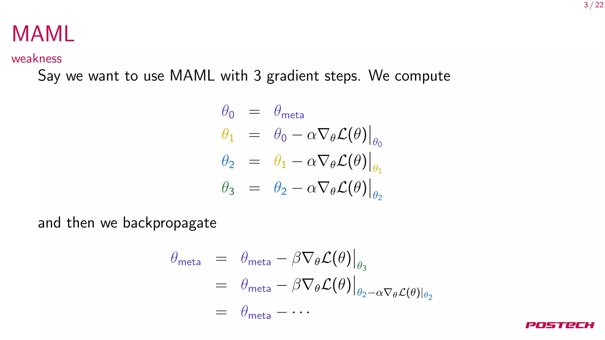
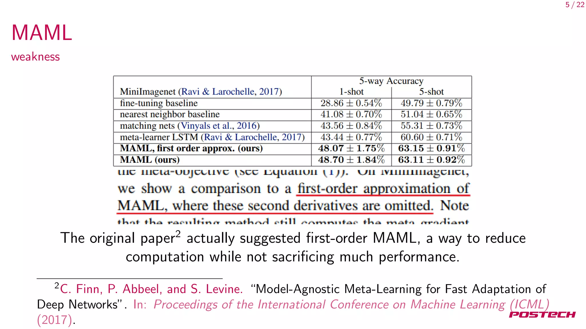
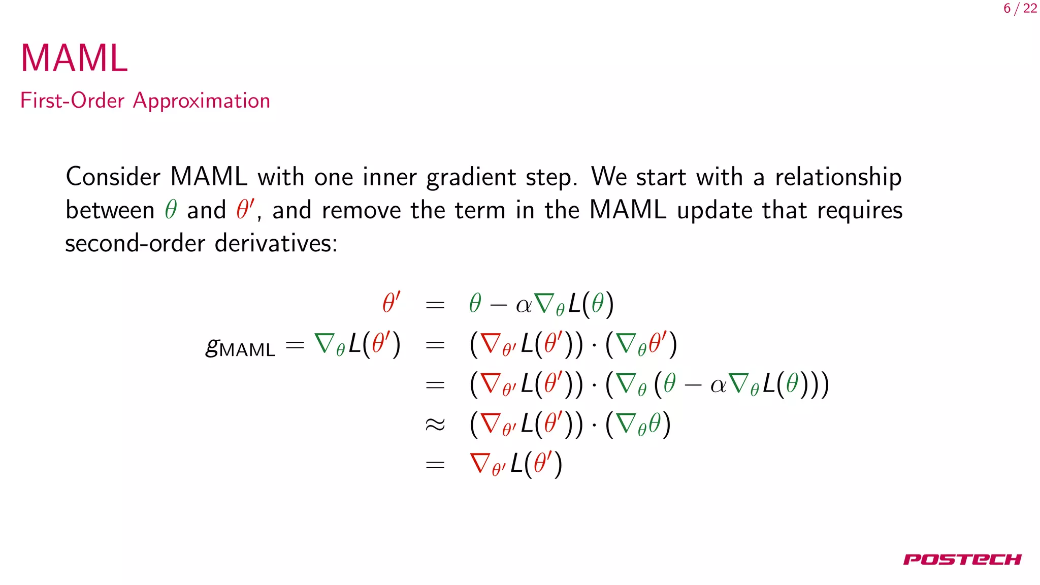
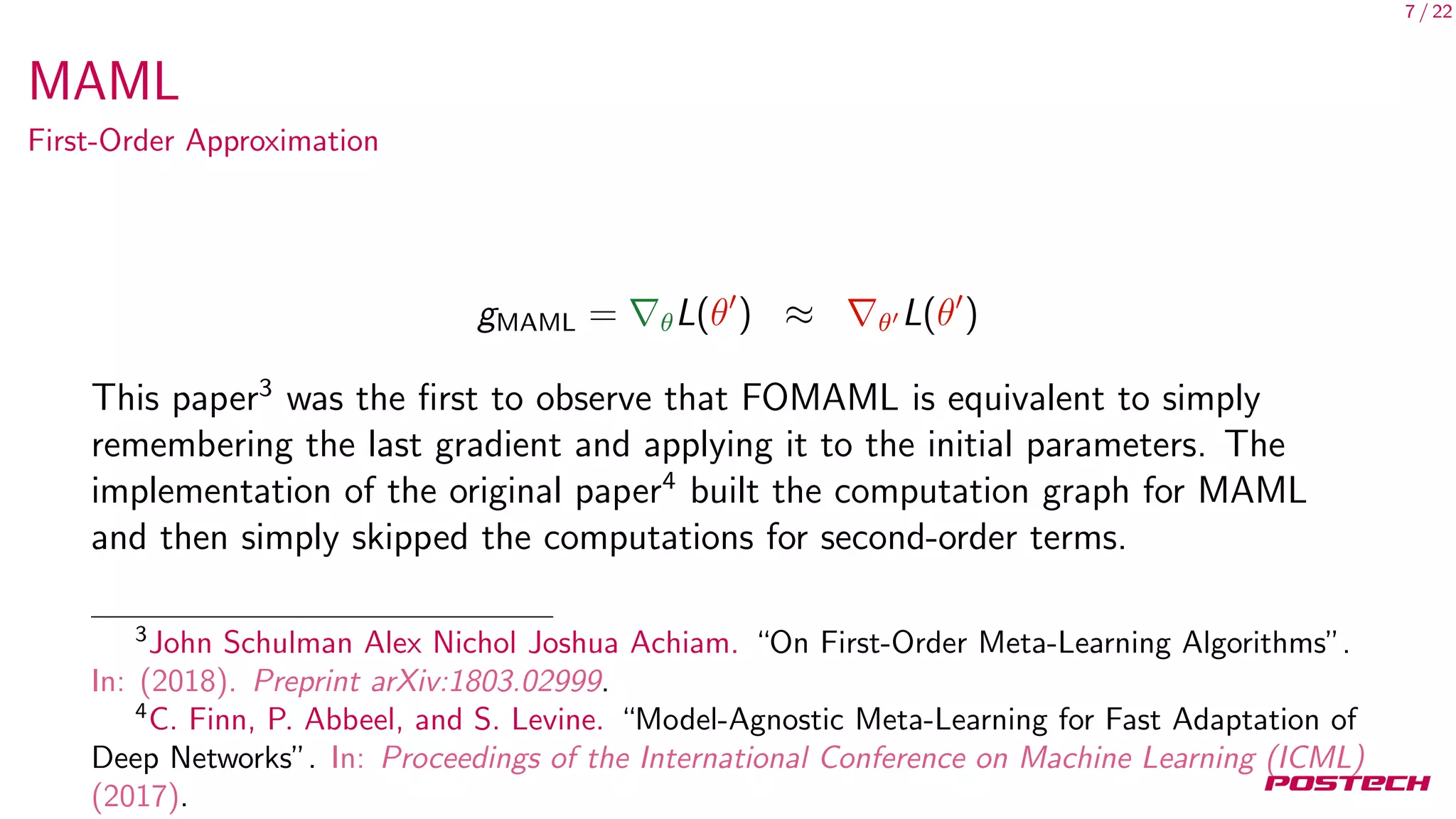
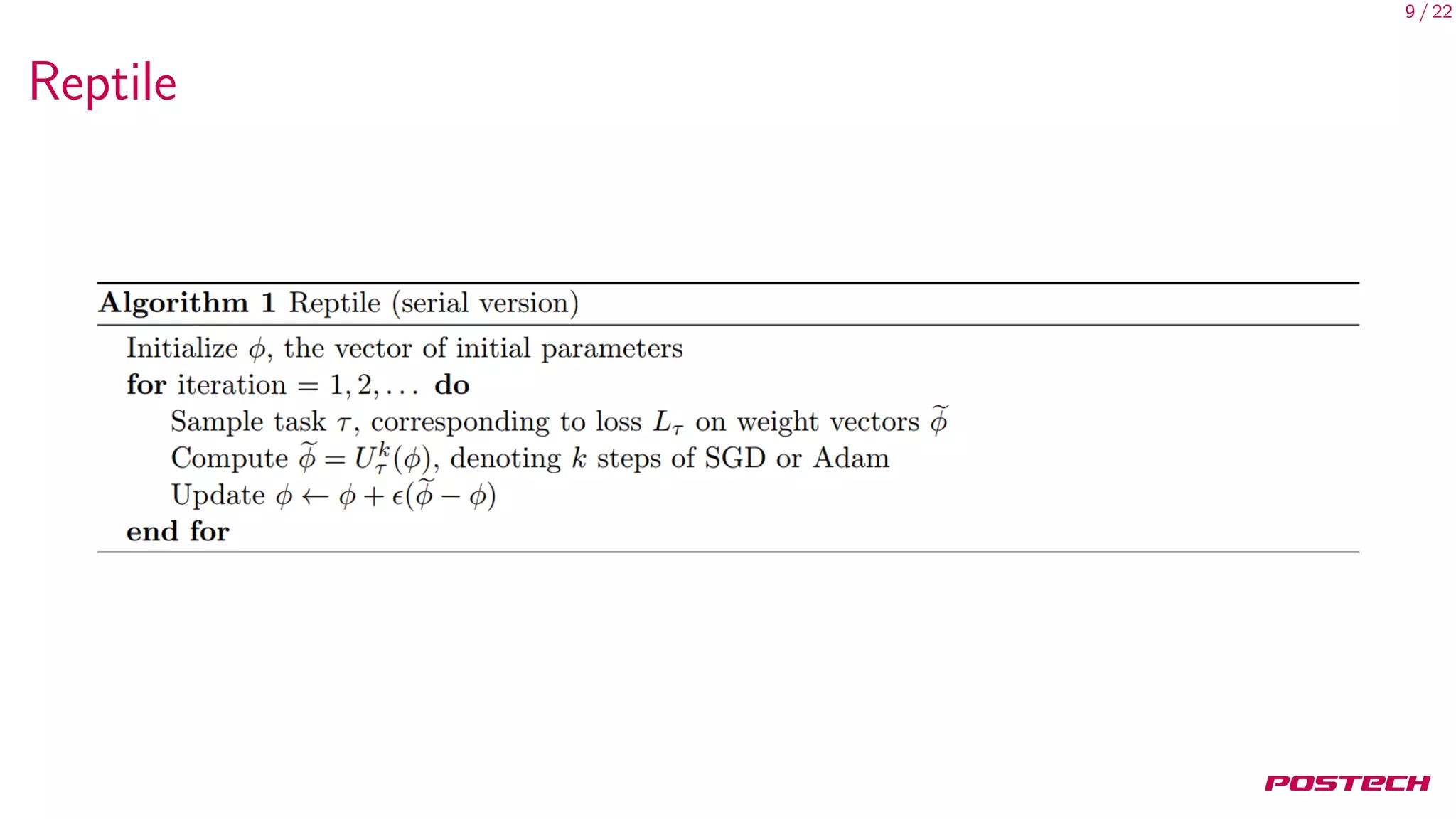
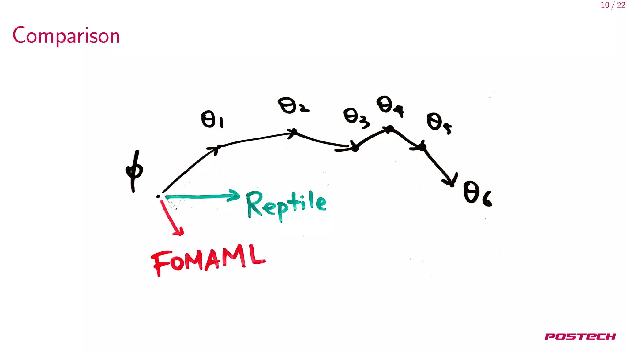
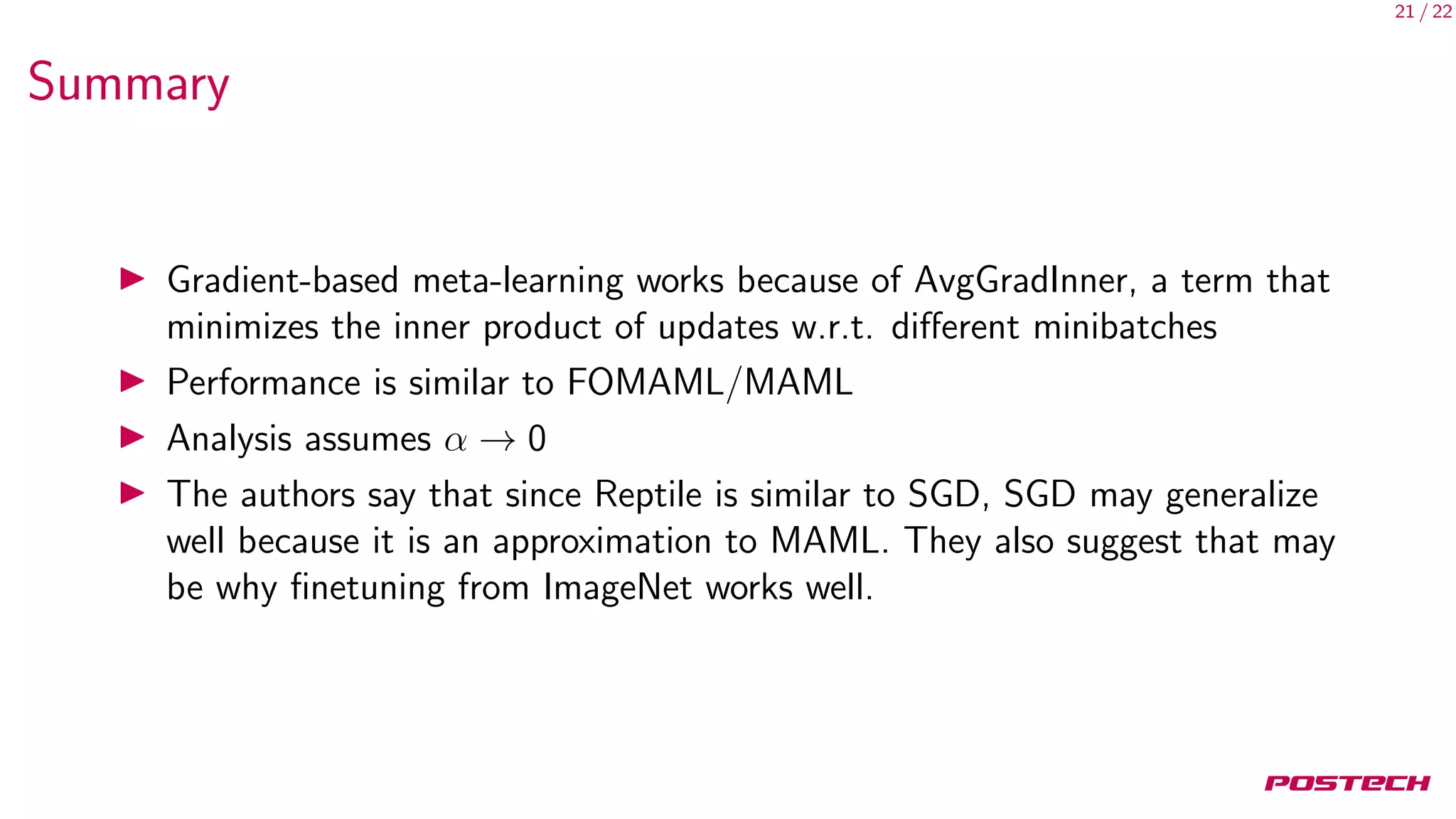
This document summarizes and analyzes first-order meta-learning algorithms. It discusses MAML, which approximates the MAML objective using only first-order information (FOMAML). FOMAML is equivalent to applying the last gradient to the initial parameters. Reptile is also analyzed, which simply averages the parameter updates. In expectation, the gradients of MAML, FOMAML and Reptile depend on the average gradient and average inner product of gradients. Experiments show similar performance between FOMAML and Reptile. The analysis suggests SGD may generalize well due to being an approximation of MAML.

1. 1 / 22
On First-Order Meta-Learning Algorithms
Yoonho Lee
Department of Computer Science and Engineering
Pohang University of Science and Technology
May 17, 2018

2. 2 / 22
MAML
1
1
C. Finn, P. Abbeel, and S. Levine. “Model-Agnostic Meta-Learning for Fast Adaptation of
Deep Networks”. In: Proceedings of the International Conference on Machine Learning (ICML)
(2017).

3. 3 / 22
MAML
weakness
Say we want to use MAML with 3 gradient steps. We compute
θ0 = θmeta
θ1 = θ0 − α θL(θ) θ0
θ2 = θ1 − α θL(θ) θ1
θ3 = θ2 − α θL(θ) θ2
and then we backpropagate
θmeta = θmeta − β θL(θ) θ3
= θmeta − β θL(θ) θ2−α θL(θ)|θ2
= θmeta − · · ·

4. 4 / 22
MAML
weakness
A weakness of MAML is that the need for memory and computation scales
linearly with the number of gradient updates.

5. 5 / 22
MAML
weakness
The original paper2
actually suggested first-order MAML, a way to reduce
computation while not sacrificing much performance.
2
C. Finn, P. Abbeel, and S. Levine. “Model-Agnostic Meta-Learning for Fast Adaptation of
Deep Networks”. In: Proceedings of the International Conference on Machine Learning (ICML)
(2017).

6. 6 / 22
MAML
First-Order Approximation
Consider MAML with one inner gradient step. We start with a relationship
between θ and θ , and remove the term in the MAML update that requires
second-order derivatives:
θ = θ − α θL(θ)
gMAML = θL(θ ) = ( θ L(θ )) · ( θθ )
= ( θ L(θ )) · ( θ (θ − α θL(θ)))
≈ ( θ L(θ )) · ( θθ)
= θ L(θ )

7. 7 / 22
MAML
First-Order Approximation
gMAML = θL(θ ) ≈ θ L(θ )
This paper3
was the first to observe that FOMAML is equivalent to simply
remembering the last gradient and applying it to the initial parameters. The
implementation of the original paper4
built the computation graph for MAML
and then simply skipped the computations for second-order terms.
3
John Schulman Alex Nichol Joshua Achiam. “On First-Order Meta-Learning Algorithms”.
In: (2018). Preprint arXiv:1803.02999.
4
C. Finn, P. Abbeel, and S. Levine. “Model-Agnostic Meta-Learning for Fast Adaptation of
Deep Networks”. In: Proceedings of the International Conference on Machine Learning (ICML)
(2017).

8. 8 / 22
On First-Order Meta-Learning Algorithms
Alex Nichol, Joshua Achiam, John Schulman

9. 9 / 22
Reptile

10. 10 / 22
Comparison

11. 11 / 22
Analysis
Definitions
We assume that we get a sequence of loss functions (L1, L2, · · · , Ln). We
introduce the following symbols for convenience:
gi = Li (φi )
¯gi = Li (φ1)
¯Hi = Li (φ1)
Ui (φ) = φ − αLi (φ)
φi+1 = φi − αgi = Ui (φi )
We want to express everything in terms of ¯gi and ¯Hi to analyze what each
update means from the point of view of the initial parameters.

12. 12 / 22
Analysis
We begin by expressing gi using ¯gi and ¯Hi :
gi = Li (φi ) = Li (φ1) + Li (φ1)(φi − φ1) + O(α2
)
= ¯gi + ¯Hi (φi − φ1) + O(α2
)
= ¯gi − α ¯Hi
i−1
j=1
gj + O(α2
)
= ¯gi − α ¯Hi
i−1
j=1
¯gj + O(α2
)

13. 13 / 22
Analysis
The MAML update is:
gMAML =
∂
∂φ1
Lk(φk)
=
∂
∂φ1
Lk(Uk−1(Uk−2(· · · (U1(φ1)))))
= U1(φ1) · · · Uk−1(φk−1)Lk(φk)
= (I − αL1(φ1)) · · · (I − αLk−1(φk−1))Lk(φk)
=
k−1
j=1
(I − αLj (φj )) gk

14. 14 / 22
Analysis
gMAML =
k−1
j=1
(I − αLj (φj )) gk
=
k−1
j=1
(I − α ¯Hj ) ¯gk − α ¯Hk
k−1
j=1
¯gj + O(α2
)
= I − α
k−1
j=1
¯Hj ¯gk − α ¯Hk
k−1
j=1
¯gj + O(α2
)
= ¯gk − α
k−1
j=1
¯Hj ¯gk − α ¯Hk
k−1
j=1
¯gj + O(α2
)

15. 15 / 22
Analysis
Assuming k = 2,
gMAML = ¯g2 − α ¯H2 ¯g1 − α ¯H1 ¯g2 + O(α2
)
gFOMAML = g2 = ¯g2 − α ¯H2 ¯g1 + O(α2
)
gReptile = g1 + g2 = ¯g1 + ¯g2 − α ¯H2 ¯g1 + O(α2
)

16. 16 / 22
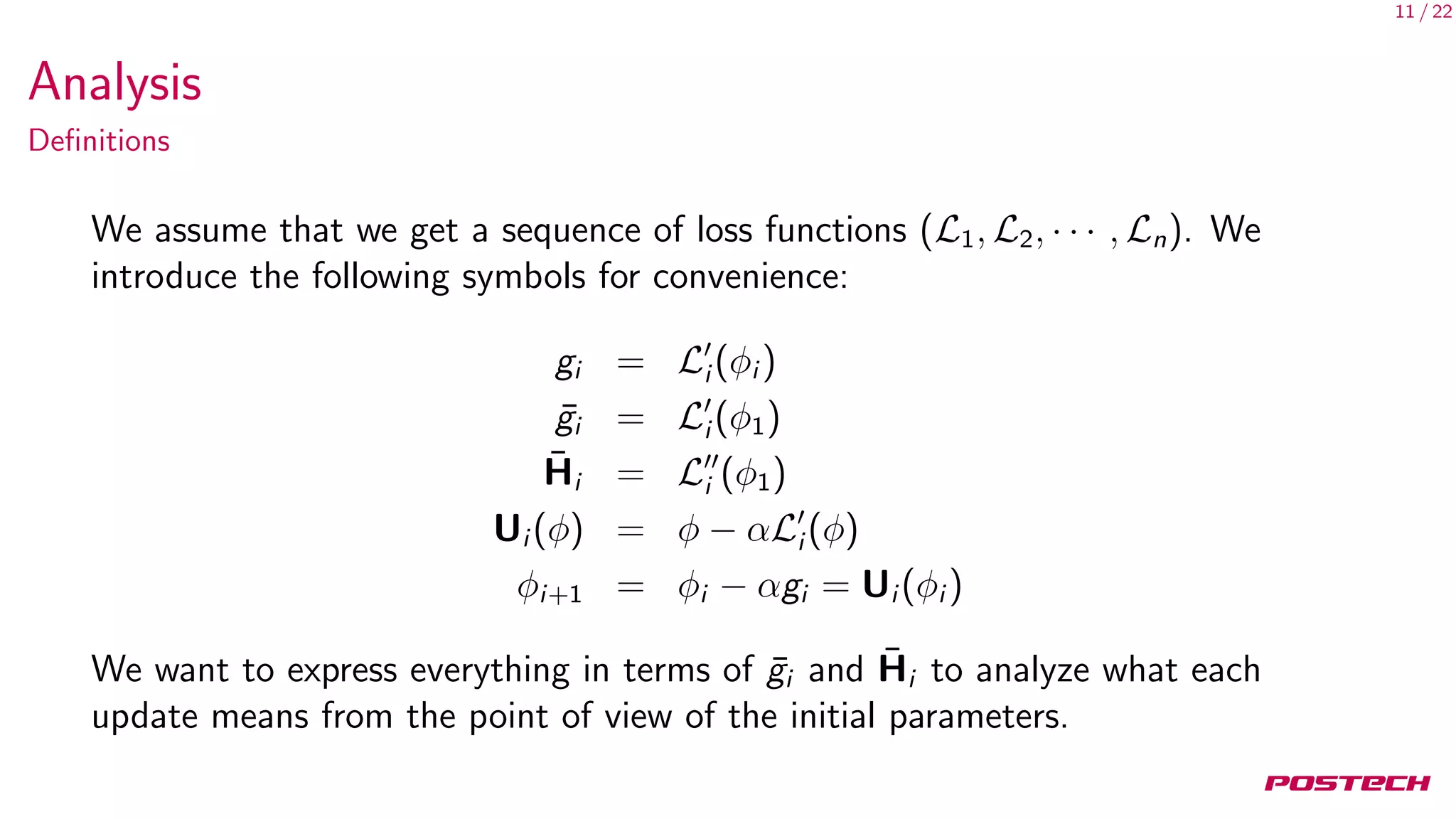
Analysis
Since loss functions are exchangeable (losses are typically computed over
minibatches randomly taken from a larger set),
E[¯g1] = E[¯g2] = · · ·
Similarly,
E[ ¯Hi ¯gj ] =
1
2
E[ ¯Hi ¯gj + ¯Hj ¯gi ]
=
1
2
E[
∂
∂φ1
(¯gi · ¯gj )]

17. 17 / 22
Analysis
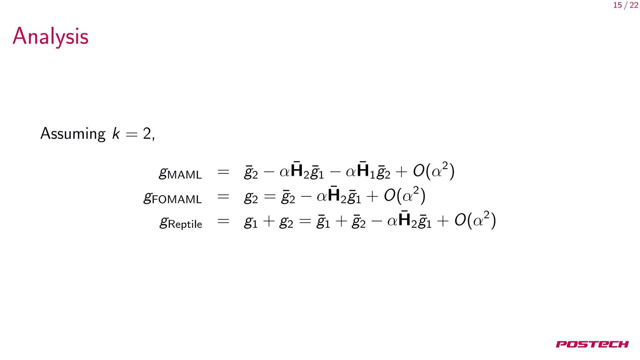
Therfore, in expectation, there are only two kinds of terms:
AvgGrad = E[¯g]
AvgGradInner = E[¯g · ¯g ]
We now return to gradient-based meta-learning for k steps:
E[gMAML] = 1AvgGrad + (2k − 2)αAvgGradInner
E[gFOMAML] = 1AvgGrad + (k − 1)αAvgGradInner
E[gReptile] = kAvgGrad +
1
2
k(k − 1)αAvgGradInner

18. 18 / 22
Experiments
Gradient Combinations

19. 19 / 22
Experiments
Few-shot Classification

20. 20 / 22
Experiments
Reptile vs FOMAML

21. 21 / 22
Summary
Gradient-based meta-learning works because of AvgGradInner, a term that
minimizes the inner product of updates w.r.t. different minibatches
Performance is similar to FOMAML/MAML
Analysis assumes α → 0
The authors say that since Reptile is similar to SGD, SGD may generalize
well because it is an approximation to MAML. They also suggest that may
be why finetuning from ImageNet works well.

22. 22 / 22
References I
[1] John Schulman Alex Nichol Joshua Achiam. “On First-Order Meta-Learning
Algorithms”. In: (2018). Preprint arXiv:1803.02999.
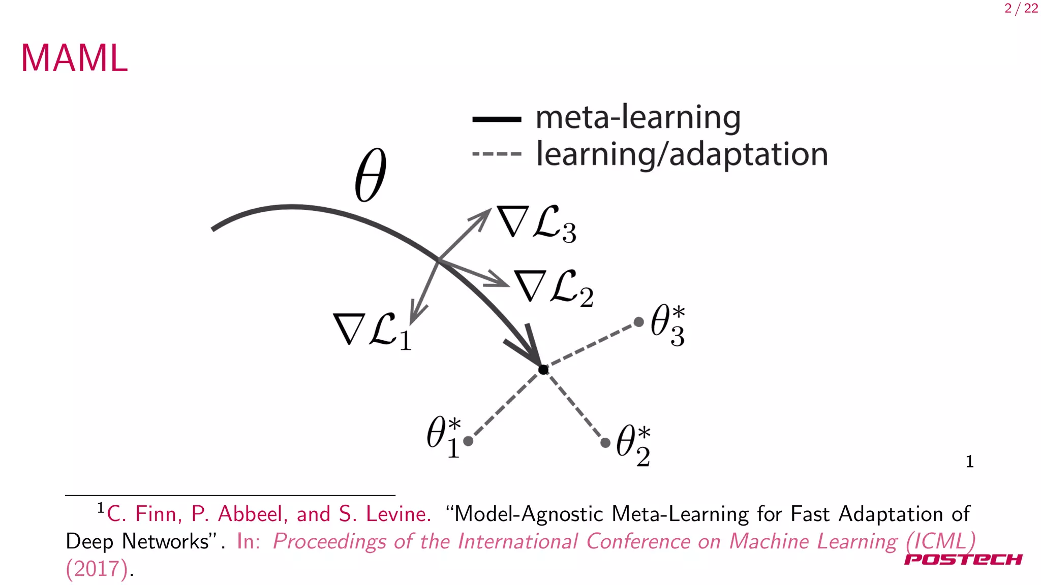
[2] C. Finn, P. Abbeel, and S. Levine. “Model-Agnostic Meta-Learning for Fast
Adaptation of Deep Networks”. In: Proceedings of the International
Conference on Machine Learning (ICML) (2017).

23. 23 / 22
Thank You