Download as PDF, PPTX

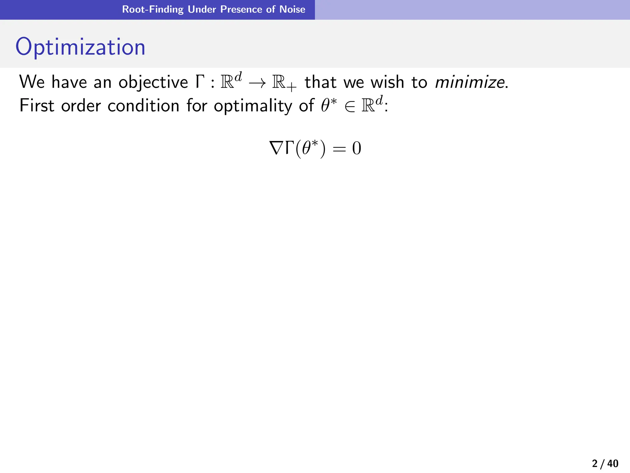
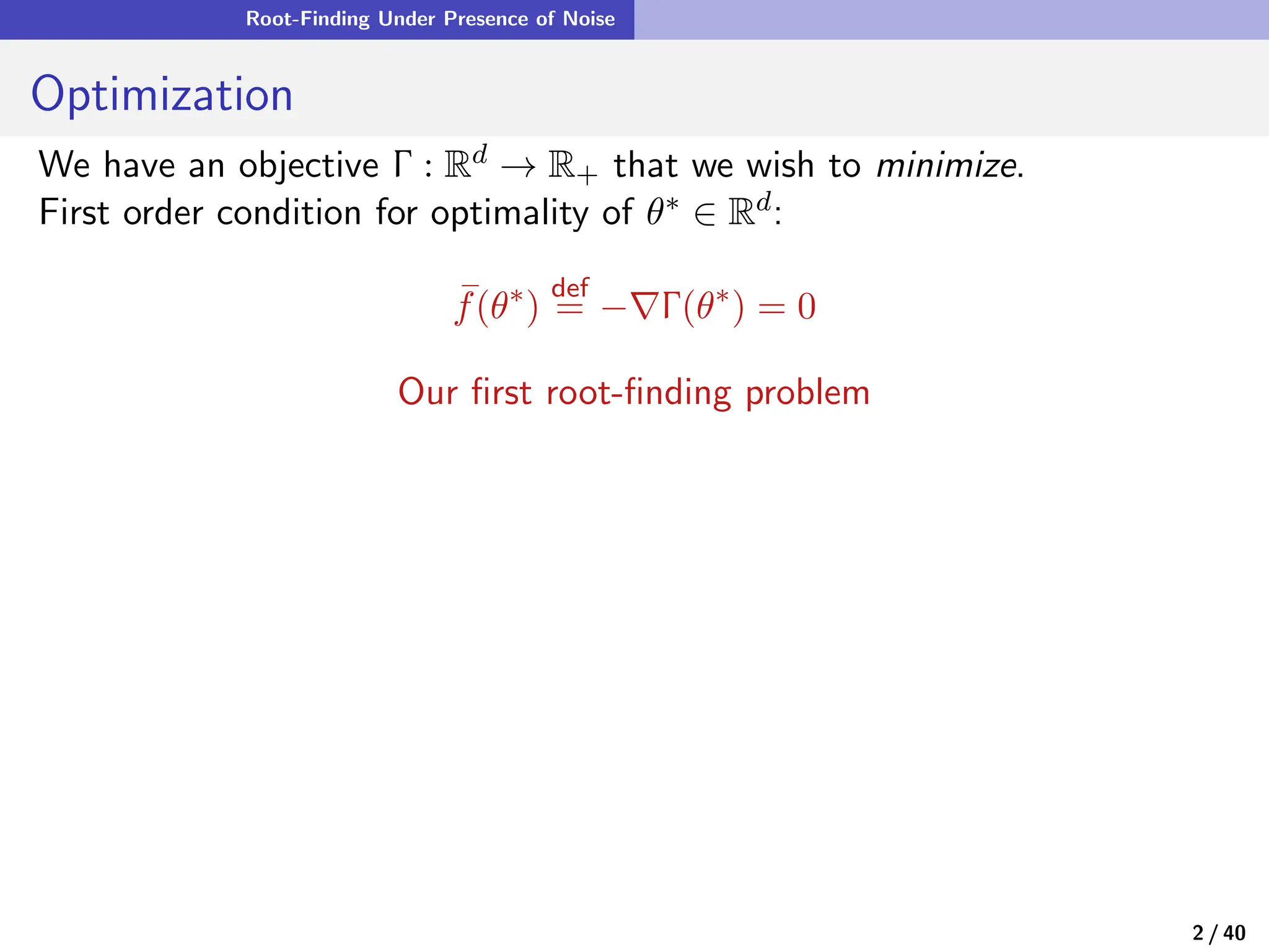
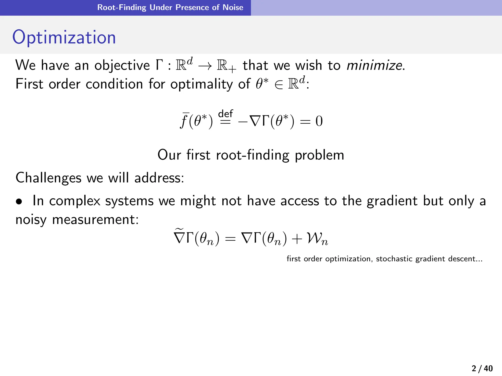

![Root-Finding Under Presence of Noise
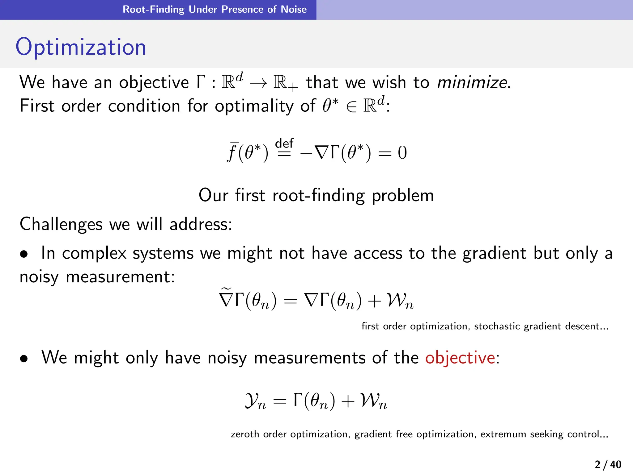
Gradient-Free Optimization
How would we estimate θopt
∈ arg min
θ
Γ if we have access to Γ for any θ?
For any fixed θ and a small ε > 0, let
f(θ, ξ) = −
1
ε
ξΓ(θ + εξ)
where ξ is zero-mean.
=⇒ s
f(θ) := E[f(θ, ξ)] approximates −∇Γ (θ)
3 / 40](https://image.slidesharecdn.com/nrelescnicerebootforne-240325183317-b7afa7f2/75/Quasi-Stochastic-Approximation-Algorithm-Design-Principles-with-Applications-to-Machine-Learning-and-Optimization-8-2048.jpg)
![Root-Finding Under Presence of Noise
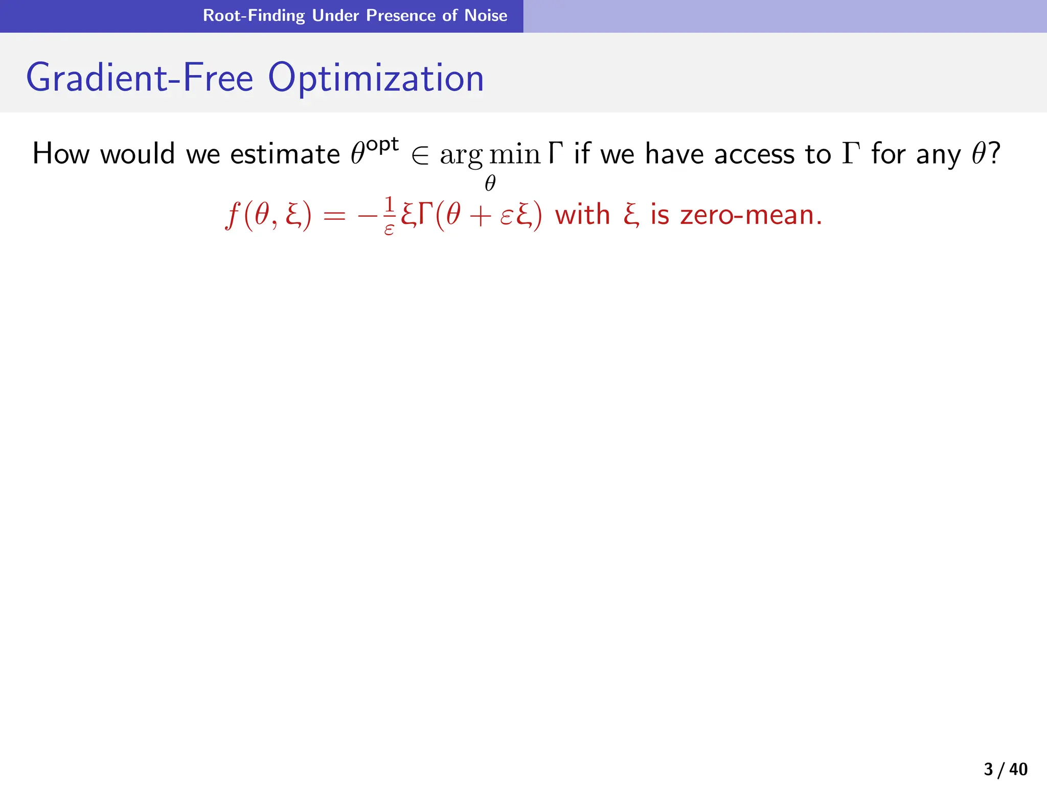
Gradient-Free Optimization
How would we estimate θopt
∈ arg min
θ
Γ if we have access to Γ for any θ?
f(θ, ξ) = −1
ε ξΓ(θ + εξ) with ξ is zero-mean.
• A bit of Taylor series...
f(θ, ξ) = −
1
ε
ξΓ(θ) − ξξ⊺
∇Γ(θ) + O(ε)
• Taking expectations of both sides yields
E[f(θ, ξ)] = −Cov(ξ)∇Γ(θ) + O(ε)
3 / 40](https://image.slidesharecdn.com/nrelescnicerebootforne-240325183317-b7afa7f2/75/Quasi-Stochastic-Approximation-Algorithm-Design-Principles-with-Applications-to-Machine-Learning-and-Optimization-11-2048.jpg)
![Root-Finding Under Presence of Noise
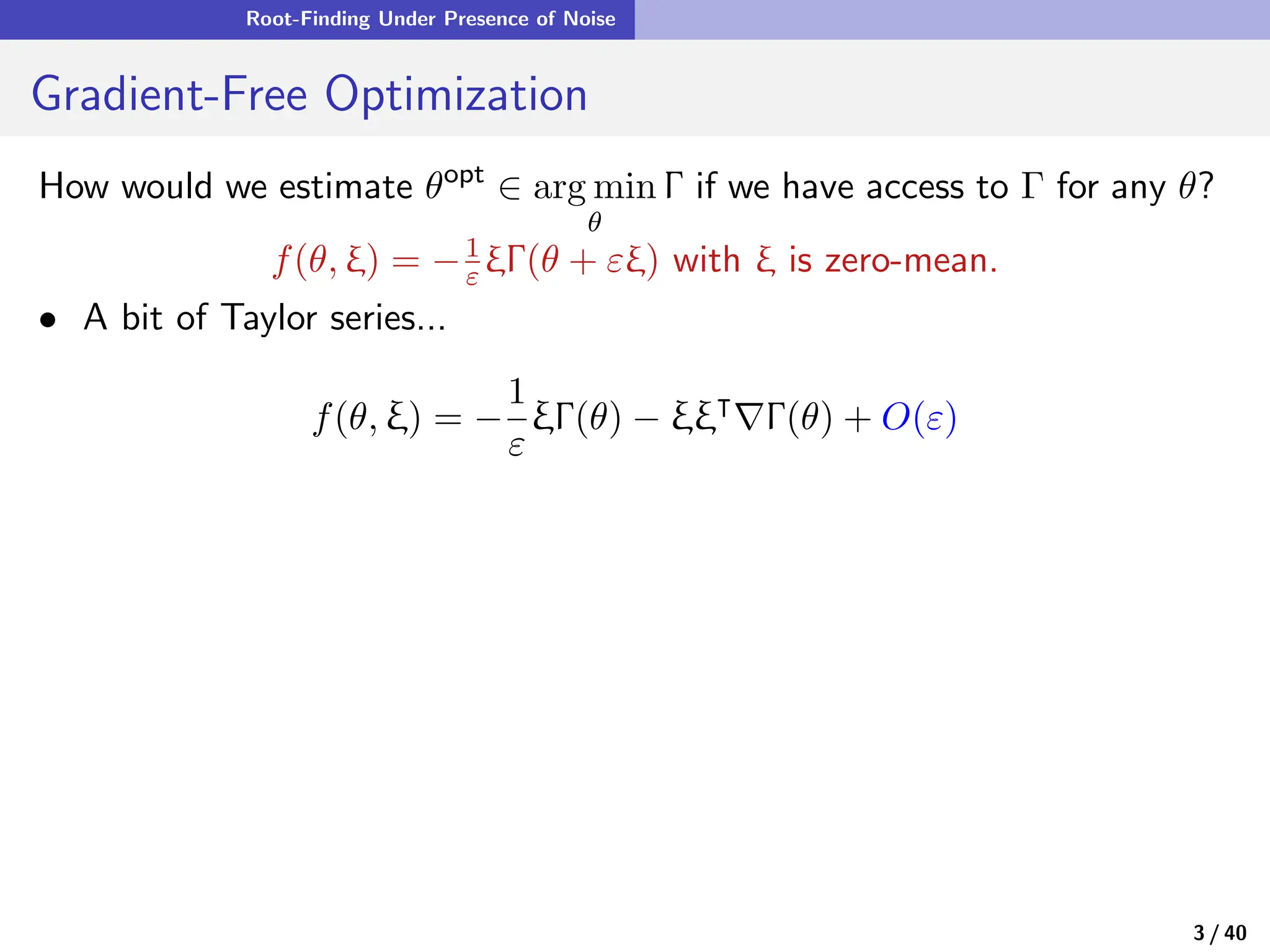
Gradient-Free Optimization
How would we estimate θopt
∈ arg min
θ
Γ if we have access to Γ for any θ?
f(θ, ξ) = −1
ε ξΓ(θ + εξ) with ξ is zero-mean.
• A bit of Taylor series...
f(θ, ξ) = −
1
ε
ξΓ(θ) − ξξ⊺
∇Γ(θ) + O(ε)
• Taking expectations of both sides yields
s
f(θ) := E[f(θ, ξ)] = −Cov(ξ)∇Γ(θ) + O(ε)
3 / 40](https://image.slidesharecdn.com/nrelescnicerebootforne-240325183317-b7afa7f2/75/Quasi-Stochastic-Approximation-Algorithm-Design-Principles-with-Applications-to-Machine-Learning-and-Optimization-12-2048.jpg)
![Root-Finding Under Presence of Noise
Gradient-Free Optimization
How would we estimate θopt
∈ arg min
θ
Γ if we have access to Γ for any θ?
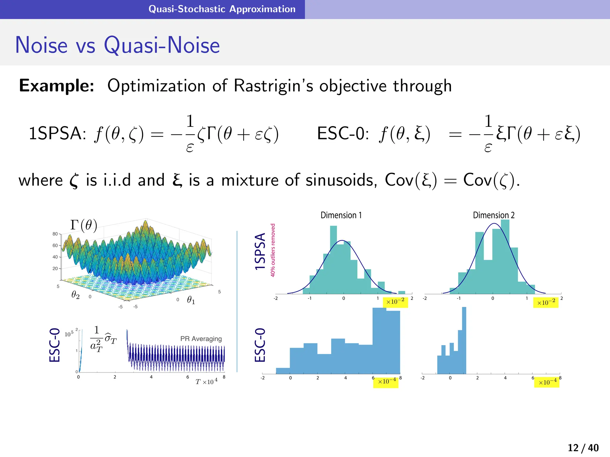
1SPSA: f(θ, ξ) = −1
ε ξΓ(θ + εξ) with ξ is zero-mean.
• A bit of Taylor series...
f(θ, ξ) = −
1
ε
ξΓ(θ) − ξξ⊺
∇Γ(θ) + O(ε)
• Taking expectations of both sides yields
s
f(θ) := E[f(θ, ξ)] = −Cov(ξ)∇Γ(θ) + O(ε)
s
f(θ∗
) = 0 , s
f(θopt
) = O(ε)
see Spall [67] and Ariyur & Krstić [3].
3 / 40](https://image.slidesharecdn.com/nrelescnicerebootforne-240325183317-b7afa7f2/75/Quasi-Stochastic-Approximation-Algorithm-Design-Principles-with-Applications-to-Machine-Learning-and-Optimization-13-2048.jpg)
![Quasi-Stochastic Approximation
Zooming Out
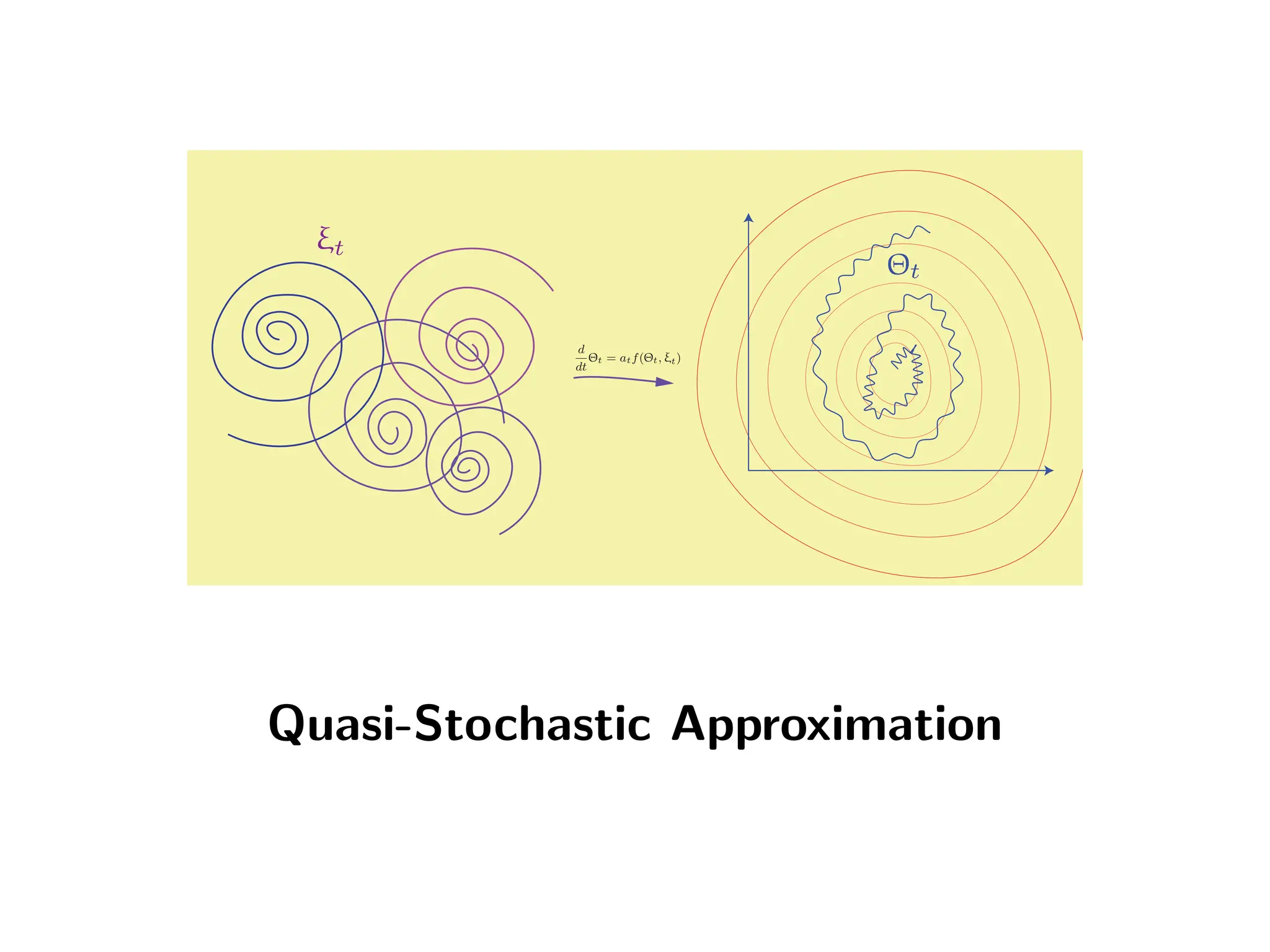
• In quasi-stochastic approximation, ξ is a smooth deterministic process,
θn+1 = θn + αn+1f(θn, ξn+1)
The probing signal ξ is typically chosen as: ξt = G(Φt) where Φ ∈ CK
with entries
Φi
t = exp(2πj[ωit + ϕi])
and {ωi} distinct.
6 / 40](https://image.slidesharecdn.com/nrelescnicerebootforne-240325183317-b7afa7f2/75/Quasi-Stochastic-Approximation-Algorithm-Design-Principles-with-Applications-to-Machine-Learning-and-Optimization-23-2048.jpg)
![Quasi-Stochastic Approximation
Zooming Out
• In quasi-stochastic approximation, ξ is a smooth deterministic process,
θn+1 = θn + αn+1f(θn, ξn+1)
The probing signal ξ is typically chosen as: ξt = G(Φt) where Φ ∈ CK
with entries
Φi
t = exp(2πj[ωit + ϕi])
and {ωi} distinct.
• Expressed as ODEs for ease of analysis,
QSA ODE: d
dt Θt = atf(Θt, ξt)
Common choices for {at} include:
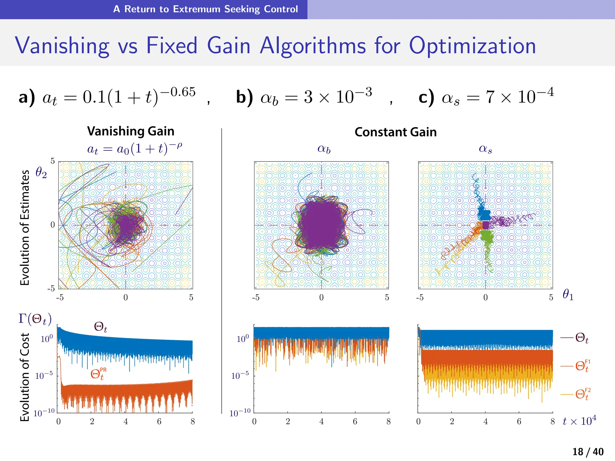
⋄ Vanishing gain: at = (t + 1)−ρ with ρ ∈ (1/2, 1)
⋄ Constant gain: at ≡ α > 0 for all t
6 / 40](https://image.slidesharecdn.com/nrelescnicerebootforne-240325183317-b7afa7f2/75/Quasi-Stochastic-Approximation-Algorithm-Design-Principles-with-Applications-to-Machine-Learning-and-Optimization-24-2048.jpg)
![Quasi-Stochastic Approximation
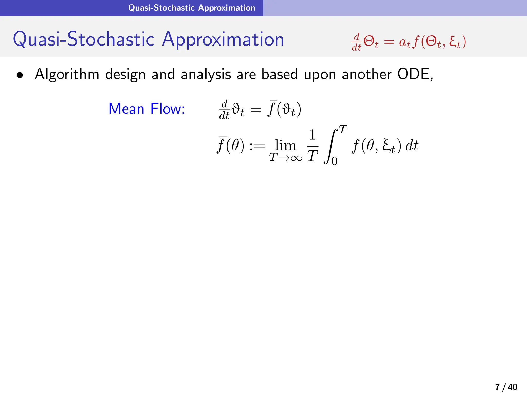
Quasi-Stochastic Approximation d
dt Θt = atf(Θt, ξt)
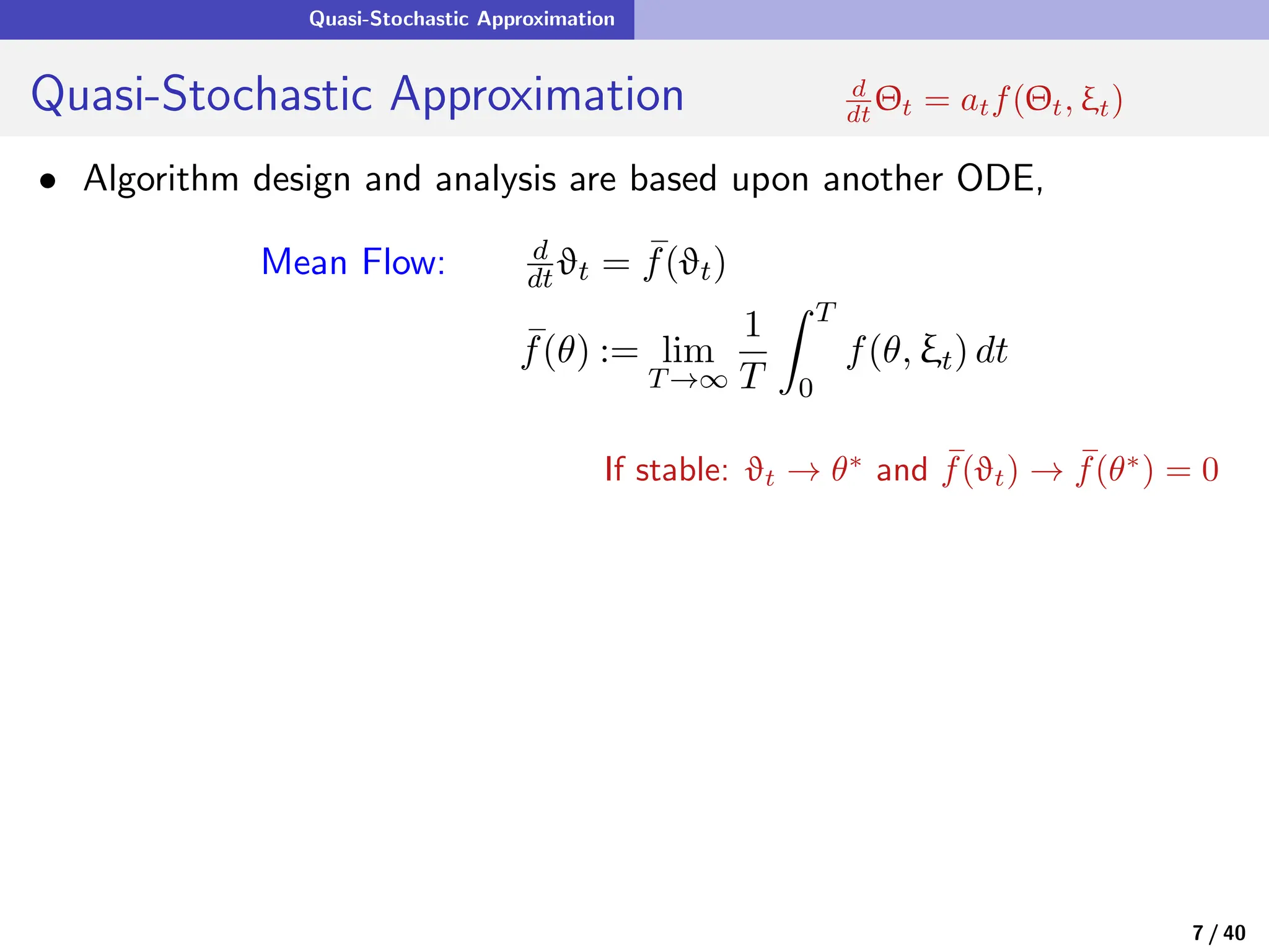
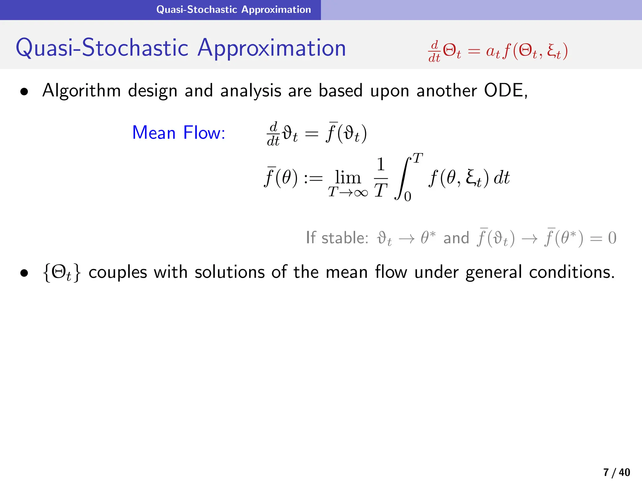
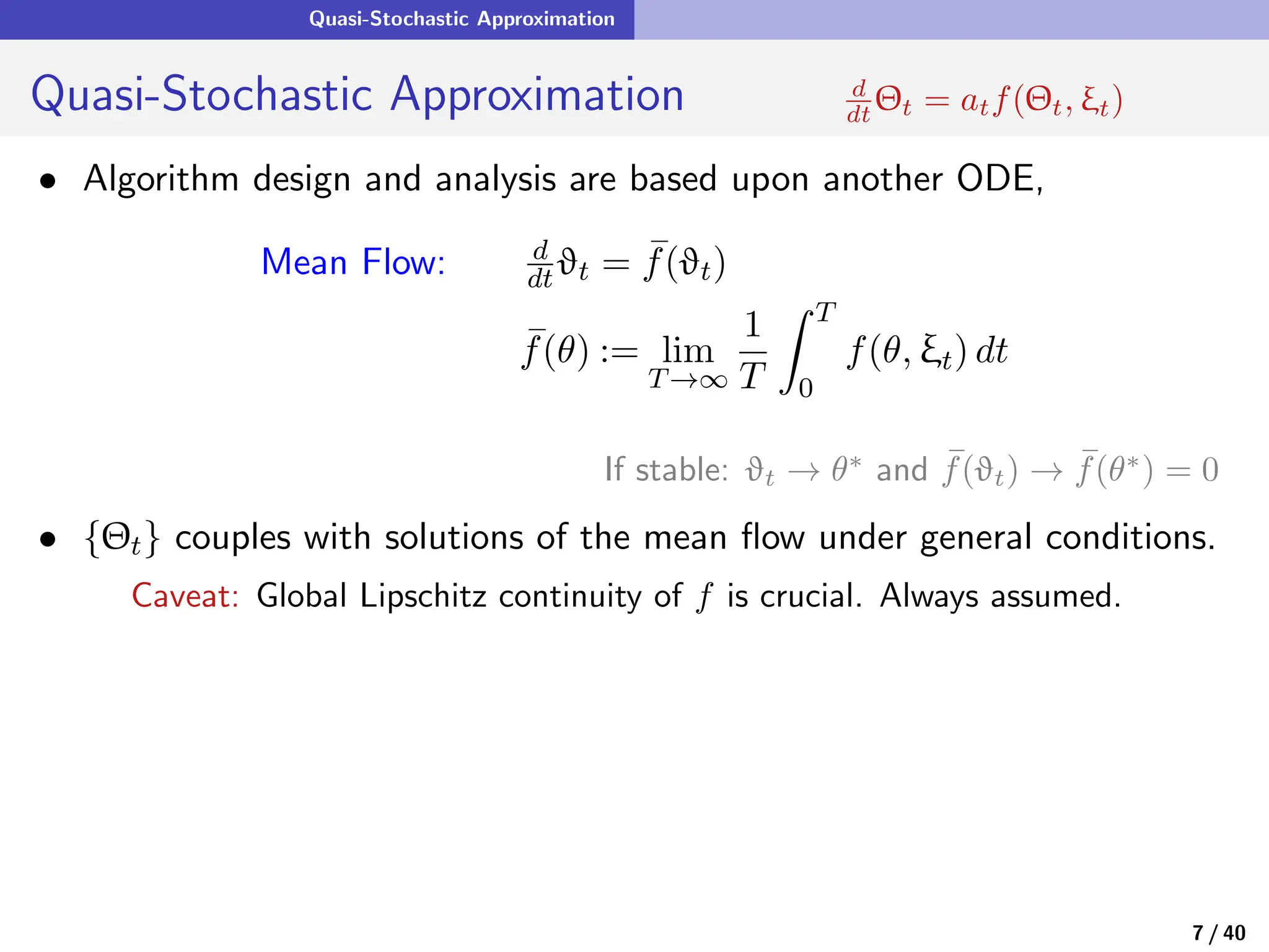
• Algorithm design and analysis are based upon another ODE,
Mean Flow: d
dt ϑt = s
f(ϑt)
s
f(θ) := lim
T→∞
1
T
Z T
0
f(θ, ξt) dt
If stable: ϑt → θ∗
and s
f(ϑt) → s
f(θ∗
) = 0
• {Θt} couples with solutions of the mean flow under general conditions.
Caveat: Global Lipschitz continuity of f is crucial. Always assumed.
• Pertubative mean flow #1:
d
dt Θt = at[ s
f(Θt) + e
Ξt] , e
Ξt := f(Θt, ξt) − s
f(Θt)
7 / 40](https://image.slidesharecdn.com/nrelescnicerebootforne-240325183317-b7afa7f2/75/Quasi-Stochastic-Approximation-Algorithm-Design-Principles-with-Applications-to-Machine-Learning-and-Optimization-29-2048.jpg)
![Quasi-Stochastic Approximation
Quasi-Stochastic Approximation d
dt Θt = atf(Θt, ξt)
• Algorithm design and analysis are based upon another ODE,
Mean Flow: d
dt ϑt = s
f(ϑt)
s
f(θ) := lim
T→∞
1
T
Z T
0
f(θ, ξt) dt
If stable: ϑt → θ∗
and s
f(ϑt) → s
f(θ∗
) = 0
• {Θt} couples with solutions of the mean flow under general conditions.
Caveat: Global Lipschitz continuity of f is crucial. Always assumed.
• Pertubative mean flow #1:
d
dt Θt = at[ s
f(Θt) + e
Ξt] , e
Ξt := f(Θt, ξt) − s
f(Θt)
Can we do any better?
7 / 40](https://image.slidesharecdn.com/nrelescnicerebootforne-240325183317-b7afa7f2/75/Quasi-Stochastic-Approximation-Algorithm-Design-Principles-with-Applications-to-Machine-Learning-and-Optimization-30-2048.jpg)
![Quasi-Stochastic Approximation
Métivier and Priouret To The Rescue!
• Pertubative mean (p-mean) flow #1:
d
dt Θt = at[ s
f(Θt) + e
Ξt] , e
Ξt := f(Θt, ξt) − s
f(Θt)
• Representation for e
Ξ based on solutions to Poisson’s equation.
First instance, solution ˆ
f with forcing function f:
d
dt
ˆ
f(θ, Φt) = −[f(θ, ξt) − s
f(θ)] , θ ∈ Rd
8 / 40](https://image.slidesharecdn.com/nrelescnicerebootforne-240325183317-b7afa7f2/75/Quasi-Stochastic-Approximation-Algorithm-Design-Principles-with-Applications-to-Machine-Learning-and-Optimization-31-2048.jpg)
![Quasi-Stochastic Approximation
Métivier and Priouret To The Rescue!
• Pertubative mean (p-mean) flow #1:
d
dt Θt = at[ s
f(Θt) + e
Ξt] , e
Ξt := f(Θt, ξt) − s
f(Θt)
• Representation for e
Ξ based on solutions to Poisson’s equation.
First instance, solution ˆ
f with forcing function f:
d
dt
ˆ
f(θ, Φt) = −[f(θ, ξt) − s
f(θ)] , θ ∈ Rd
=⇒ d
dt
ˆ
f(Θt, Φt) = −e
Ξt + ∂θ
ˆ
f(Θt, Φt) · d
dt Θt
8 / 40](https://image.slidesharecdn.com/nrelescnicerebootforne-240325183317-b7afa7f2/75/Quasi-Stochastic-Approximation-Algorithm-Design-Principles-with-Applications-to-Machine-Learning-and-Optimization-32-2048.jpg)
![Quasi-Stochastic Approximation
Métivier and Priouret To The Rescue!
• Pertubative mean (p-mean) flow #1:
d
dt Θt = at[ s
f(Θt) + e
Ξt] , e
Ξt := f(Θt, ξt) − s
f(Θt)
• Representation for e
Ξ based on solutions to Poisson’s equation.
First instance, solution ˆ
f with forcing function f:
d
dt
ˆ
f(θ, Φt) = −[f(θ, ξt) − s
f(θ)] , θ ∈ Rd
=⇒ d
dt
ˆ
f(Θt, Φt) = −e
Ξt + ∂θ
ˆ
f(Θt, Φt)[atf(Θt, ξt)]
e
Ξt = zero mean + small
8 / 40](https://image.slidesharecdn.com/nrelescnicerebootforne-240325183317-b7afa7f2/75/Quasi-Stochastic-Approximation-Algorithm-Design-Principles-with-Applications-to-Machine-Learning-and-Optimization-33-2048.jpg)
![Quasi-Stochastic Approximation
Métivier and Priouret To The Rescue!
• Pertubative mean (p-mean) flow #1:
d
dt Θt = at[ s
f(Θt) + e
Ξt] , e
Ξt := f(Θt, ξt) − s
f(Θt)
• Representation for e
Ξ based on solutions to Poisson’s equation.
First instance, solution ˆ
f with forcing function f:
d
dt
ˆ
f(θ, Φt) = −[f(θ, ξt) − s
f(θ)] , θ ∈ Rd
=⇒ d
dt
ˆ
f(Θt, Φt) = −e
Ξt + ∂θ
ˆ
f(Θt, Φt)[atf(Θt, ξt)]
e
Ξt = zero mean + small
• Borrowed from the stochastic approximation literature:
disturbance decomposition introduced by Métivier and Priouret.
8 / 40](https://image.slidesharecdn.com/nrelescnicerebootforne-240325183317-b7afa7f2/75/Quasi-Stochastic-Approximation-Algorithm-Design-Principles-with-Applications-to-Machine-Learning-and-Optimization-34-2048.jpg)
![Quasi-Stochastic Approximation
Perturbative Mean Flow
The perturbative mean (p-mean) flow representation
d
dt Θt = at[ s
f(Θt) + e
Ξt]
e
Ξt = −at
s
Υ(Θt) +
2
X
i=0
a2−i
t
di
dti
Wi
t
where {s
Υt, Wi
t : i = 0, 1, 2} are smooth deterministic functions of (Θt, Φt)
admitting representations in terms of solutions to Poisson’s equation.
• Opens doors for analysis: transient bounds and filter design.
9 / 40](https://image.slidesharecdn.com/nrelescnicerebootforne-240325183317-b7afa7f2/75/Quasi-Stochastic-Approximation-Algorithm-Design-Principles-with-Applications-to-Machine-Learning-and-Optimization-35-2048.jpg)
![Quasi-Stochastic Approximation
Perturbative Mean Flow
The perturbative mean (p-mean) flow representation
d
dt Θt = at[ s
f(Θt) + e
Ξt]
e
Ξt = −at
s
Υ(Θt) +
2
X
i=0
a2−i
t
di
dti
Wi
t
where {s
Υt, Wi
t : i = 0, 1, 2} are smooth deterministic functions of (Θt, Φt)
admitting representations in terms of solutions to Poisson’s equation.
• Opens doors for analysis: transient bounds and filter design.
What is s
Υ? It appears with multiplicative noise:
s
Υ(θ) := − lim
T→∞
1
T
Z T
0
∂θ
ˆ
f(θ, Φt)f(θ, ξt) dt
9 / 40](https://image.slidesharecdn.com/nrelescnicerebootforne-240325183317-b7afa7f2/75/Quasi-Stochastic-Approximation-Algorithm-Design-Principles-with-Applications-to-Machine-Learning-and-Optimization-36-2048.jpg)
![Quasi-Stochastic Approximation
Convergence and Acceleration d
dt Θt = atf(Θt, ξt)
• When at = (1 + t)−ρ with ρ ∈ (1/2, 1),
Θt = θ∗
+ at[A∗
]−1 s
Υ∗
+ nicet
o
⇒ ∥Θt − θ∗
∥2
= O(a2
t )
where s
Υ∗ = s
Υ(θ∗) and A∗ = ∂θ
s
f(θ∗).
10 / 40](https://image.slidesharecdn.com/nrelescnicerebootforne-240325183317-b7afa7f2/75/Quasi-Stochastic-Approximation-Algorithm-Design-Principles-with-Applications-to-Machine-Learning-and-Optimization-37-2048.jpg)
![Quasi-Stochastic Approximation
Convergence and Acceleration d
dt Θt = atf(Θt, ξt)
• When at = (1 + t)−ρ with ρ ∈ (1/2, 1),
Θt = θ∗
+ at[A∗
]−1 s
Υ∗
+ nicet
o
⇒ ∥Θt − θ∗
∥2
= O(a2
t )
where s
Υ∗ = s
Υ(θ∗) and A∗ = ∂θ
s
f(θ∗).
• Convergence is accelerated through Polyak-Ruppert (PR) averaging
ΘPR
T =
1
T − δT
Z T
δT
Θt dt , δ ∈ (0, 1)
10 / 40](https://image.slidesharecdn.com/nrelescnicerebootforne-240325183317-b7afa7f2/75/Quasi-Stochastic-Approximation-Algorithm-Design-Principles-with-Applications-to-Machine-Learning-and-Optimization-38-2048.jpg)
![Quasi-Stochastic Approximation
Convergence and Acceleration d
dt Θt = atf(Θt, ξt)
• When at = (1 + t)−ρ with ρ ∈ (1/2, 1),
Θt = θ∗
+ at[A∗
]−1 s
Υ∗
+ nicet
o
⇒ ∥Θt − θ∗
∥2
= O(a2
t )
where s
Υ∗ = s
Υ(θ∗) and A∗ = ∂θ
s
f(θ∗).
• Convergence is accelerated through Polyak-Ruppert (PR) averaging
ΘPR
T =
1
T − δT
Z T
δT
Θt dt , δ ∈ (0, 1)
• Extremely fast rates are obtained:
ΘPR
T = θ∗
+ O(aT ∥s
Υ∗
∥) + O(a2
T ) ⇒ ∥ΘPR
T − θ∗
∥2
= O(a4
T )
| {z }
If s
Υ∗=0
10 / 40](https://image.slidesharecdn.com/nrelescnicerebootforne-240325183317-b7afa7f2/75/Quasi-Stochastic-Approximation-Algorithm-Design-Principles-with-Applications-to-Machine-Learning-and-Optimization-39-2048.jpg)
![Quasi-Stochastic Approximation
Killing s
Υ∗
Φi
t = exp(2πj[ωit + ϕi])
Clever Probing design
⋄ Design ξ so that ξt = G(Φt) with G analytic and choose frequencies
{ω1 , . . . , ωK} satisfying,
ωi = log(ai/bi) > 0 , {ai, bi} positive integers.
11 / 40](https://image.slidesharecdn.com/nrelescnicerebootforne-240325183317-b7afa7f2/75/Quasi-Stochastic-Approximation-Algorithm-Design-Principles-with-Applications-to-Machine-Learning-and-Optimization-40-2048.jpg)
![Quasi-Stochastic Approximation
Killing s
Υ∗
Φi
t = exp(2πj[ωit + ϕi])
Clever Probing design
⋄ Design ξ so that ξt = G(Φt) with G analytic and choose frequencies
{ω1 , . . . , ωK} satisfying,
ωi = log(ai/bi) > 0 , {ai, bi} positive integers.
Cleverness # 1: existence of solutions to Poisson’s equation.
• Solutions can be represented as sums of integrals
Z t
0
exp(2πj[ω◦
t + ϕ◦
]) dt
ω◦ = n1ω1 + · · · nKωK.
=⇒ Require bounds on 1/ω◦
11 / 40](https://image.slidesharecdn.com/nrelescnicerebootforne-240325183317-b7afa7f2/75/Quasi-Stochastic-Approximation-Algorithm-Design-Principles-with-Applications-to-Machine-Learning-and-Optimization-41-2048.jpg)
![Quasi-Stochastic Approximation
Killing s
Υ∗
Φi
t = exp(2πj[ωit + ϕi])
Clever Probing design
⋄ Design ξ so that ξt = G(Φt) with G analytic and choose frequencies
{ω1 , . . . , ωK} satisfying,
ωi = log(ai/bi) > 0 , {ai, bi} positive integers.
Cleverness # 1: existence of solutions to Poisson’s equation.
• Solutions can be represented as sums of integrals
Z t
0
exp(2πj[ω◦
t + ϕ◦
]) dt
ω◦ = n1ω1 + · · · nKωK.
=⇒ Require bounds on 1/ω◦
Great lower bounds on |ω◦| from Baker’s Theorem.
11 / 40](https://image.slidesharecdn.com/nrelescnicerebootforne-240325183317-b7afa7f2/75/Quasi-Stochastic-Approximation-Algorithm-Design-Principles-with-Applications-to-Machine-Learning-and-Optimization-42-2048.jpg)
![Quasi-Stochastic Approximation
Killing s
Υ∗
Φi
t = exp(2πj[ωit + ϕi])
Clever Probing design
⋄ Design ξ so that ξt = G(Φt) with G analytic and choose frequencies
{ω1 , . . . , ωK} satisfying,
ωi = log(ai/bi) > 0 , {ai, bi} positive integers.
Cleverness # 1: existence of solutions to Poisson’s equation.
• Solutions can be represented as sums of integrals
=⇒ Require bounds on 1/ω◦
Great lower bounds on |ω◦| from Baker’s Theorem.
Cleverness # 2: ĝ ⊥ h for smooth functions g, h of the probing signal.
11 / 40](https://image.slidesharecdn.com/nrelescnicerebootforne-240325183317-b7afa7f2/75/Quasi-Stochastic-Approximation-Algorithm-Design-Principles-with-Applications-to-Machine-Learning-and-Optimization-43-2048.jpg)
![Quasi-Stochastic Approximation
Killing s
Υ∗
Φi
t = exp(2πj[ωit + ϕi])
Clever Probing design
⋄ Design ξ so that ξt = G(Φt) with G analytic and choose frequencies
{ω1 , . . . , ωK} satisfying,
ωi = log(ai/bi) > 0 , {ai, bi} positive integers.
Cleverness # 1: existence of solutions to Poisson’s equation.
• Solutions can be represented as sums of integrals
=⇒ Require bounds on 1/ω◦
Great lower bounds on |ω◦| from Baker’s Theorem.
Cleverness # 2: ĝ ⊥ h for smooth functions g, h of the probing signal.
s
Υi(θ) =
X
j
⟨ĝi,j, hj⟩, with g = ∂θf and h = f.
11 / 40](https://image.slidesharecdn.com/nrelescnicerebootforne-240325183317-b7afa7f2/75/Quasi-Stochastic-Approximation-Algorithm-Design-Principles-with-Applications-to-Machine-Learning-and-Optimization-44-2048.jpg)
![Quasi-Stochastic Approximation
Killing s
Υ∗
Φi
t = exp(2πj[ωit + ϕi])
Clever Probing design
⋄ Design ξ so that ξt = G(Φt) with G analytic and choose frequencies
{ω1 , . . . , ωK} satisfying,
ωi = log(ai/bi) > 0 , {ai, bi} positive integers.
Cleverness # 1: existence of solutions to Poisson’s equation.
• Solutions can be represented as sums of integrals
=⇒ Require bounds on 1/ω◦
Great lower bounds on |ω◦| from Baker’s Theorem.
Cleverness # 2: ĝ ⊥ h for smooth functions g, h of the probing signal.
s
Υi(θ) =
X
j
⟨ĝi,j, hj⟩, with g = ∂θf and h = f.
= 0
11 / 40](https://image.slidesharecdn.com/nrelescnicerebootforne-240325183317-b7afa7f2/75/Quasi-Stochastic-Approximation-Algorithm-Design-Principles-with-Applications-to-Machine-Learning-and-Optimization-45-2048.jpg)
![Quasi-Stochastic Approximation
Fixed Gain Algorithms for QSA
• The QSA ODE with fixed gain is old news! (recall the averaging principle)
d
dt Θt = αf(Θt, ξt) , α > 0
see Khalil [24].
13 / 40](https://image.slidesharecdn.com/nrelescnicerebootforne-240325183317-b7afa7f2/75/Quasi-Stochastic-Approximation-Algorithm-Design-Principles-with-Applications-to-Machine-Learning-and-Optimization-47-2048.jpg)
![Quasi-Stochastic Approximation
Fixed Gain Algorithms for QSA
• The QSA ODE with fixed gain is old news! (recall the averaging principle)
d
dt Θt = αf(Θt, ξt) , α > 0
see Khalil [24].
• Motivation is tracking: { s
ft} ⇒ {θ∗
t }
13 / 40](https://image.slidesharecdn.com/nrelescnicerebootforne-240325183317-b7afa7f2/75/Quasi-Stochastic-Approximation-Algorithm-Design-Principles-with-Applications-to-Machine-Learning-and-Optimization-48-2048.jpg)
![Quasi-Stochastic Approximation
Fixed Gain Algorithms for QSA
• The QSA ODE with fixed gain is old news! (recall the averaging principle)
d
dt Θt = αf(Θt, ξt) , α > 0
see Khalil [24].
• Motivation is tracking: { s
ft} ⇒ {θ∗
t }
• Without averaging, MSE is
lim sup
t→∞
∥Θt − θ∗
∥2
= O(α2
)
13 / 40](https://image.slidesharecdn.com/nrelescnicerebootforne-240325183317-b7afa7f2/75/Quasi-Stochastic-Approximation-Algorithm-Design-Principles-with-Applications-to-Machine-Learning-and-Optimization-49-2048.jpg)
![Quasi-Stochastic Approximation
Fixed Gain Algorithms for QSA
• The QSA ODE with fixed gain is old news! (recall the averaging principle)
d
dt Θt = αf(Θt, ξt) , α > 0
see Khalil [24].
• Motivation is tracking: { s
ft} ⇒ {θ∗
t }
• Without averaging, MSE is
lim sup
t→∞
∥Θt − θ∗
∥2
= O(α2
)
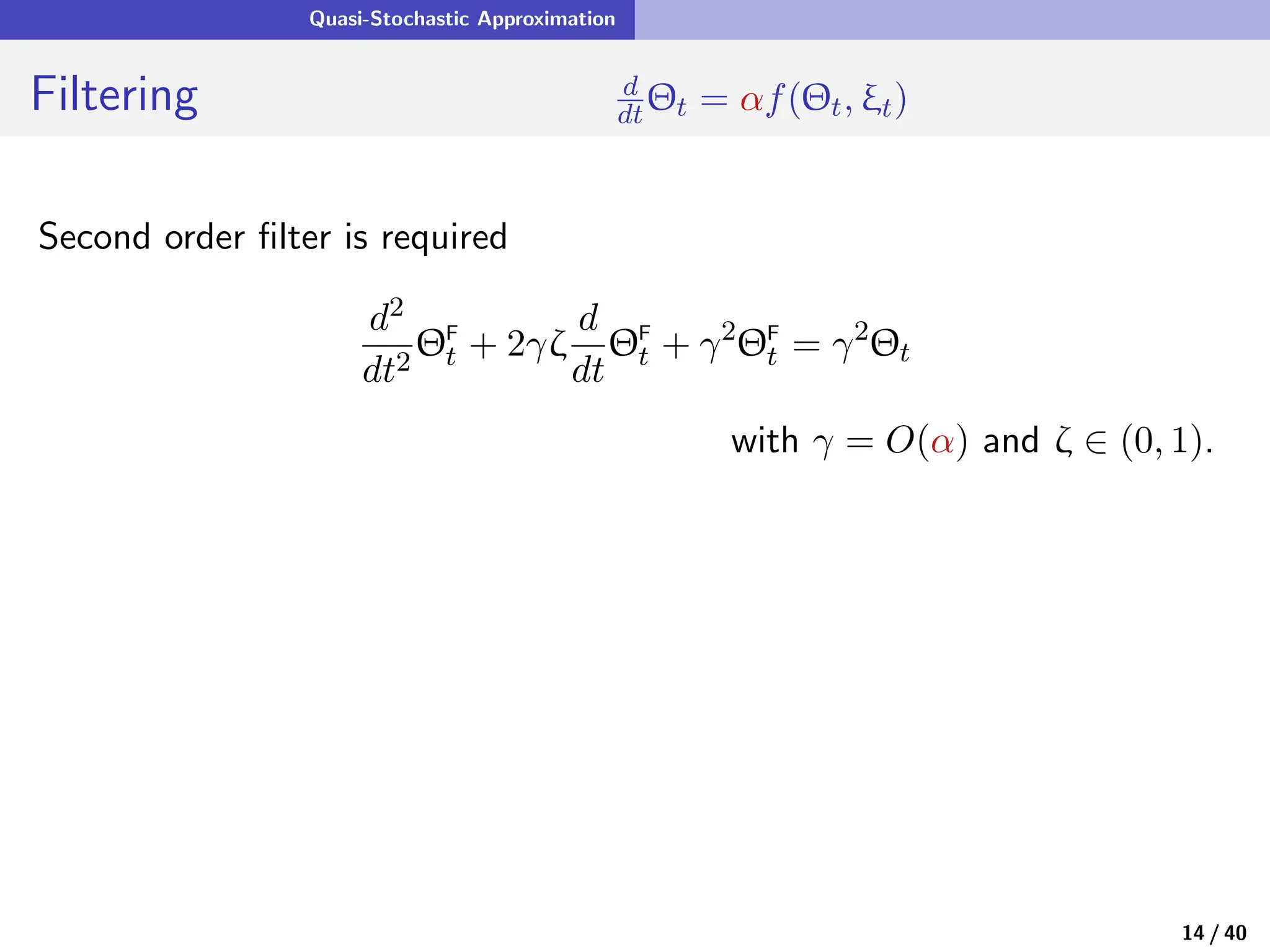
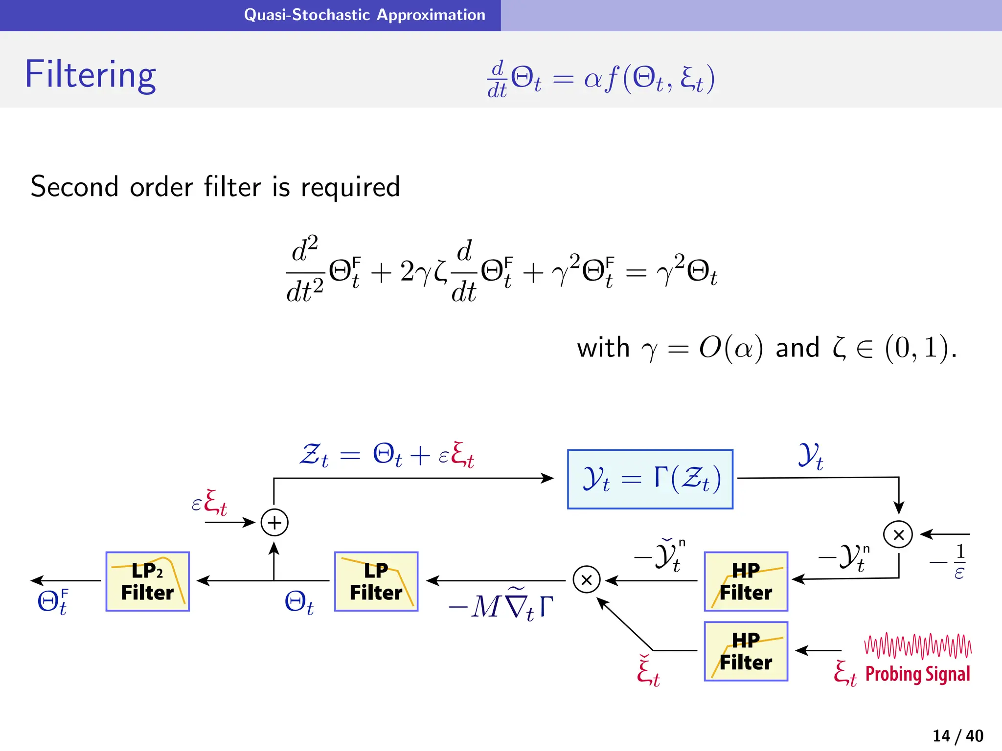
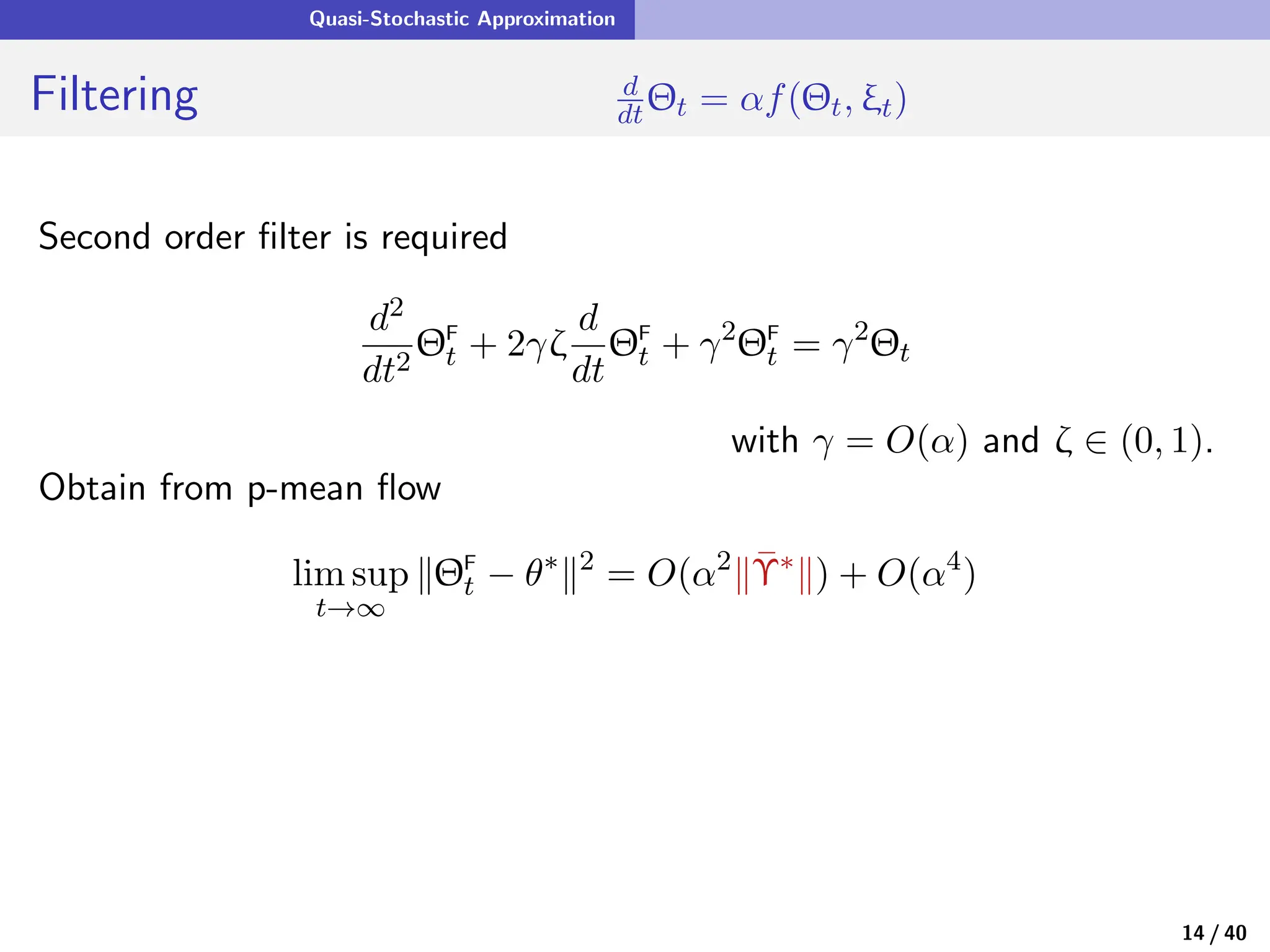
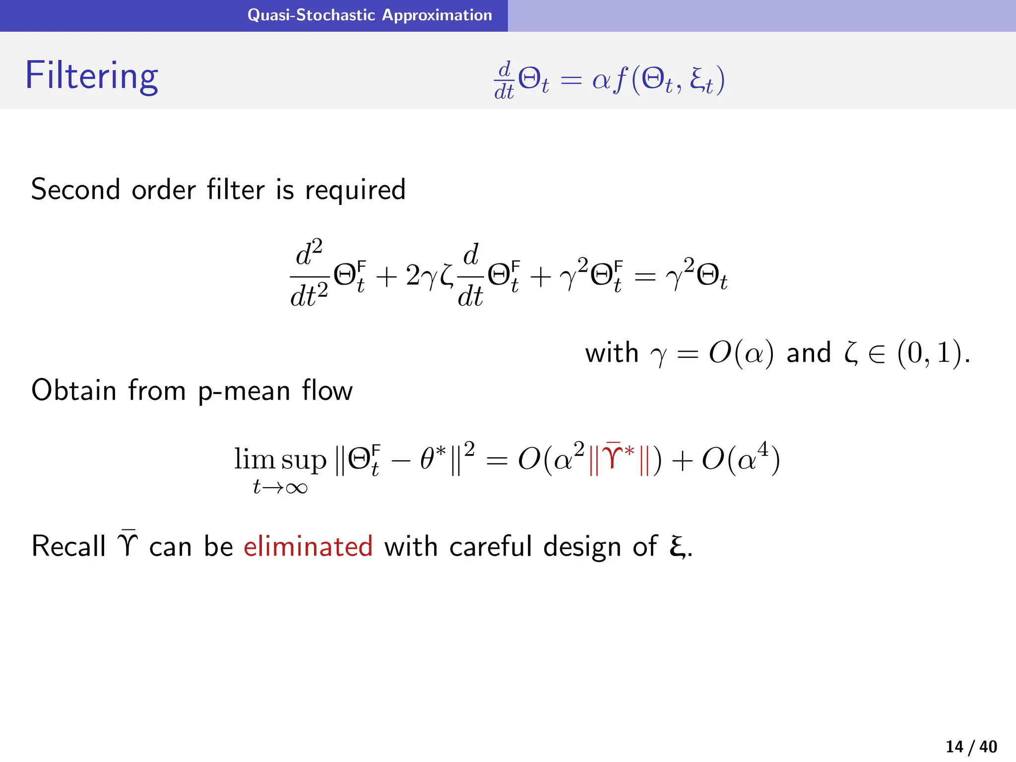
• A p-mean flow representation inspires a low pass filter to obtain
lim sup
t→∞
∥ΘF
t − θ∗
∥2
= O(α4
)
13 / 40](https://image.slidesharecdn.com/nrelescnicerebootforne-240325183317-b7afa7f2/75/Quasi-Stochastic-Approximation-Algorithm-Design-Principles-with-Applications-to-Machine-Learning-and-Optimization-50-2048.jpg)


![A Return to Extremum Seeking Control
Lipschitz Continuity Matters! f(θ, ξ) = − 1
ϵ(θ) ξΓ(θ + ϵ(θ)ξ)
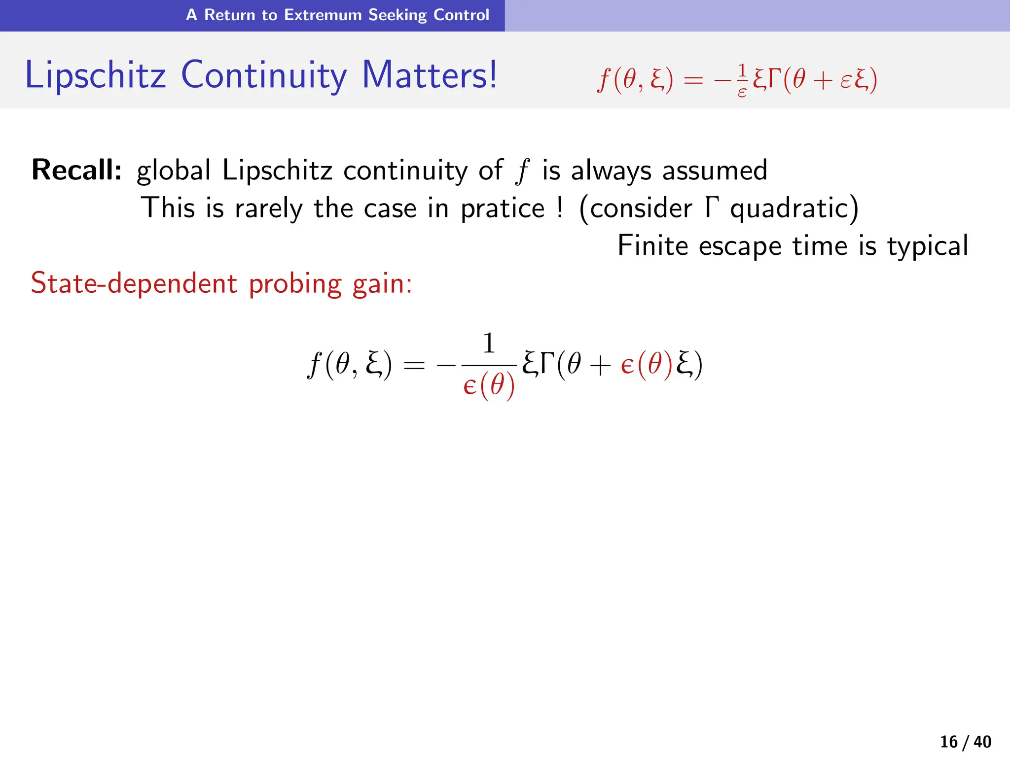
Recall: global Lipschitz continuity of f is always assumed
This is rarely the case in pratice ! (consider Γ quadratic)
Finite escape time is typical
State-dependent probing gain:
f(θ, ξ) = −
1
ϵ(θ)
ξΓ(θ + ϵ(θ)ξ)
Examples: ϵ(θ) = ε
p
1 + Γ(θ) [WLOG Γ ≥ 0]
16 / 40](https://image.slidesharecdn.com/nrelescnicerebootforne-240325183317-b7afa7f2/75/Quasi-Stochastic-Approximation-Algorithm-Design-Principles-with-Applications-to-Machine-Learning-and-Optimization-60-2048.jpg)
![A Return to Extremum Seeking Control
Lipschitz Continuity Matters! f(θ, ξ) = − 1
ϵ(θ) ξΓ(θ + ϵ(θ)ξ)
Recall: global Lipschitz continuity of f is always assumed
This is rarely the case in pratice ! (consider Γ quadratic)
Finite escape time is typical
State-dependent probing gain:
f(θ, ξ) = −
1
ϵ(θ)
ξΓ(θ + ϵ(θ)ξ)
Examples: ϵ(θ) = ε
p
1 + Γ(θ) [WLOG Γ ≥ 0]
ϵ(θ) = ε
q
1 + ∥θ − θctr∥2/σ2
p
16 / 40](https://image.slidesharecdn.com/nrelescnicerebootforne-240325183317-b7afa7f2/75/Quasi-Stochastic-Approximation-Algorithm-Design-Principles-with-Applications-to-Machine-Learning-and-Optimization-61-2048.jpg)
![A Return to Extremum Seeking Control
Lipschitz Continuity Matters! f(θ, ξ) = − 1
ϵ(θ) ξΓ(θ + ϵ(θ)ξ)
Recall: global Lipschitz continuity of f is always assumed
This is rarely the case in pratice ! (consider Γ quadratic)
Finite escape time is typical
State-dependent probing gain:
f(θ, ξ) = −
1
ϵ(θ)
ξΓ(θ + ϵ(θ)ξ)
Examples: ϵ(θ) = ε
p
1 + Γ(θ) [WLOG Γ ≥ 0]
ϵ(θ) = ε
q
1 + ∥θ − θctr∥2/σ2
p
• The algorithm is globally stable
subject to coercivity of Γ ⊕ Lipschitz gradient
• It makes sense to explore more when Γ(θ) is big!
16 / 40](https://image.slidesharecdn.com/nrelescnicerebootforne-240325183317-b7afa7f2/75/Quasi-Stochastic-Approximation-Algorithm-Design-Principles-with-Applications-to-Machine-Learning-and-Optimization-62-2048.jpg)
![Appendices
Assumptions for QSA
(A1)
VG: The process a is non-negative, monotonically decreasing, and
lim
t→∞
at = 0,
Z ∞
0
ar dr = ∞.
BG: For all t, the gain process satisfies at ≡ α > 0 for some
0 < α < α0 < 1.
(A2) The functions s
f and f are Lipschitz continuous: for a constant
Lf < ∞,
∥ s
f(θ′
) − s
f(θ)∥ ≤ Lf ∥θ′
− θ∥,
∥f(θ′
, ξ) − f(θ, ξ)∥ + ∥f(θ, ξ′
) − f(θ, ξ)∥ ≤ Lf [∥θ′
− θ∥ + ∥ξ′
− ξ∥] ,
θ′
, θ ∈ Rd
, ξ, ξ′
∈ Rm
21 / 40](https://image.slidesharecdn.com/nrelescnicerebootforne-240325183317-b7afa7f2/75/Quasi-Stochastic-Approximation-Algorithm-Design-Principles-with-Applications-to-Machine-Learning-and-Optimization-68-2048.jpg)
![Appendices
Assumptions for QSA
(A3) The ODE d
dtϑt = s
f(ϑt) is globally asymptotically stable with unique
equilibrium θ∗. Moreover, one of the following conditions holds:
(a) There is a Lipschitz continuous Lyapunov function V : Rd → R+, a
constant δ0 > 0 and a compact set S such that ∇V (ϑt) · s
f(ϑt) ≤
−δ0∥ϑt∥ whenever ϑt /
∈ S.
(b) The scaled vector field s
f∞ : Rd → Rd defined by s
f∞(θ) :=
limc→∞
s
f(cθ)/c, θ ∈ Rd, exists as a continuous function. Moreover,
the ODE@∞ defined by d
dt xt = s
f∞(xt) is globally asymptotically sta-
ble [48, §4.8.4].
(A4) The vector field s
f is differentiable, with derivative denoted Ā(θ) =
∂θ
s
f (θ).
That is, Ā(θ) is a d × d matrix for each θ ∈ Rd, with Āi,j(θ) =
∂
∂θj
s
fi (θ).
Moreover, the derivative Ā is Lipschitz continuous, and Ā∗ = Ā(θ∗) is
Hurwitz.
22 / 40](https://image.slidesharecdn.com/nrelescnicerebootforne-240325183317-b7afa7f2/75/Quasi-Stochastic-Approximation-Algorithm-Design-Principles-with-Applications-to-Machine-Learning-and-Optimization-69-2048.jpg)
![Appendices
Assumptions for QSA
(A5) Φ is the state process for a dynamical system d
dt Φt = H(Φt), H :
Ω → Ω with unique invariant measure π. It satisfies the following ergodic
theorems for the functions of interest, for each initial condition Φ0 ∈ Ω:
(i) For each θ there exists a solution ˆ
f(θ, · ) to Poisson’s equation with
forcing function f. That is,
ˆ
f(θ, Φt0 ) =
Z t1
t0
[f(θ, ξt) − s
f(θ)] dt + ˆ
f(θ, Φt1 ) , 0 ≤ t0 ≤ t1
and for each θ,
R
Ω
ˆ
f(θ, z) π(dz) = 0. Finally, ˆ
f is continuously
differentiable (C1) on Rd × Ω. Its Jacobian with respect to θ is
denoted
b
A(θ, z) := ∂θ
ˆ
f(θ, z)
where
Z
Ω
b
A(θ, z) π(dz) = 0 for each θ ∈ Rd
23 / 40](https://image.slidesharecdn.com/nrelescnicerebootforne-240325183317-b7afa7f2/75/Quasi-Stochastic-Approximation-Algorithm-Design-Principles-with-Applications-to-Machine-Learning-and-Optimization-70-2048.jpg)
![Appendices
Assumptions for QSA
(ii) For each θ, there are C1 solutions to Poisson’s equation with forcing
functions ˆ
f and Υ. They are denoted
ˆ
ˆ
f and b
Υ, respectively, satisfying
ˆ
ˆ
f(θ, Φt0 ) =
Z t1
t0
ˆ
f(θ, ξt) dt +
ˆ
ˆ
f(θ, Φt1 )
b
Υ(θ, Φt0 ) =
Z t1
t0
[Υ(θ, Φt) − s
Υ(θ)] dt + b
Υ(θ, Φt1 ) , 0 ≤ t0 ≤ t1
with s
Υ(θ) = −
Z
Ω
b
A(θ, z)f(θ, G(z)) π(dz)
Moreover, for each θ,
Z
Ω
ˆ
ˆ
f(θ, z) π(dz) =
Z
Ω
b
Υ(θ, z) π(dz) = 0
24 / 40](https://image.slidesharecdn.com/nrelescnicerebootforne-240325183317-b7afa7f2/75/Quasi-Stochastic-Approximation-Algorithm-Design-Principles-with-Applications-to-Machine-Learning-and-Optimization-71-2048.jpg)
![References
References I
[1] L. Amerio and G. Prouse.
Almost-periodic functions and functional equations.
Springer Science & Business Media, 2013.
[2] K. B. Ariyur and M. Krstić.
Analysis and design of multivariable extremum seeking.
In American Control Conference, volume 4, pages 2903–2908. IEEE, 2002.
[3] K. B. Ariyur and M. Krstić.
Real Time Optimization by Extremum Seeking Control.
John Wiley & Sons, Inc., New York, NY, 2003.
[4] S. Asmussen and P. W. Glynn.
Stochastic Simulation: Algorithms and Analysis, volume 57 of Stochastic Modelling and
Applied Probability.
Springer-Verlag, New York, 2007.
[5] A. Benveniste, M. Métivier, and P. Priouret.
Adaptive algorithms and stochastic approximations, volume 22.
Springer Science & Business Media, Berlin Heidelberg, 2012.
25 / 40](https://image.slidesharecdn.com/nrelescnicerebootforne-240325183317-b7afa7f2/75/Quasi-Stochastic-Approximation-Algorithm-Design-Principles-with-Applications-to-Machine-Learning-and-Optimization-72-2048.jpg)
![References
References II
[6] D. P. Bertsekas.
Reinforcement learning and optimal control.
Athena Scientific, Belmont, MA, 2019.
[7] S. Bhatnagar, M. C. Fu, S. I. Marcus, and I.-J. Wang.
Two-timescale simultaneous perturbation stochastic approximation using deterministic
perturbation sequences.
ACM Transactions on Modeling and Computer Simulation (TOMACS), 13(2):180–209,
2003.
[8] H. Bohr.
Almost periodic functions.
Courier Dover Publications (Reprint of the 1947 edition, Chelsea Publishing Company),
2018.
[9] V. Borkar, S. Chen, A. Devraj, I. Kontoyiannis, and S. Meyn.
The ODE method for asymptotic statistics in stochastic approximation and reinforcement
learning.
arXiv e-prints:2110.14427, pages 1–50, 2021.
[10] V. S. Borkar.
Stochastic Approximation: A Dynamical Systems Viewpoint.
Hindustan Book Agency, Delhi, India, 2nd edition, 2021.
26 / 40](https://image.slidesharecdn.com/nrelescnicerebootforne-240325183317-b7afa7f2/75/Quasi-Stochastic-Approximation-Algorithm-Design-Principles-with-Applications-to-Machine-Learning-and-Optimization-73-2048.jpg)
![References
References III
[11] V. S. Borkar and S. P. Meyn.
The ODE method for convergence of stochastic approximation and reinforcement learning.
SIAM J. Control Optim., 38(2):447–469, 2000.
[12] S. Chen, A. Devraj, A. Bernstein, and S. Meyn.
Accelerating optimization and reinforcement learning with quasi stochastic approximation.
In Proc. of the American Control Conf., pages 1965–1972, May 2021.
[13] S. Chen, A. Devraj, A. Bernstein, and S. Meyn.
Revisiting the ODE method for recursive algorithms: Fast convergence using quasi
stochastic approximation.
Journal of Systems Science and Complexity, 34(5):1681–1702, 2021.
[14] X. Chen, Y. Tang, and N. Li.
Improve single-point zeroth-order optimization using high-pass and low-pass filters.
In International Conference on Machine Learning, pages 3603–3620. PMLR, 2022.
[15] A. M. Devraj, A. Bušić, and S. Meyn.
Fundamental design principles for reinforcement learning algorithms.
In K. G. Vamvoudakis, Y. Wan, F. L. Lewis, and D. Cansever, editors, Handbook on
Reinforcement Learning and Control, Studies in Systems, Decision and Control series
(SSDC, volume 325). Springer, 2021.
27 / 40](https://image.slidesharecdn.com/nrelescnicerebootforne-240325183317-b7afa7f2/75/Quasi-Stochastic-Approximation-Algorithm-Design-Principles-with-Applications-to-Machine-Learning-and-Optimization-74-2048.jpg)
![References
References IV
[16] J. Dippon.
Accelerated randomized stochastic optimization.
The Annals of Statistics, 31(4):1260–1281, 2003.
[17] J. Dippon and J. Renz.
Weighted means in stochastic approximation of minima.
SIAM Journal on Control and Optimization, 35(5):1811–1827, 1997.
[18] C. S. Draper and Y. T. Li.
Principles of optimalizing control systems and an application to the internal combustion
engine.
American Society of Mechanical Engineers, 1951.
[19] A. Durmus, E. Moulines, A. Naumov, S. Samsonov, K. Scaman, and H.-T. Wai.
Tight high probability bounds for linear stochastic approximation with fixed step-size.
Advances in Neural Information Processing Systems and arXiv:2106.01257,
34:30063–30074, 2021.
[20] V. Fabian.
On the choice of design in stochastic approximation methods.
The Annals of Mathematical Statistics, pages 457–465, 1968.
28 / 40](https://image.slidesharecdn.com/nrelescnicerebootforne-240325183317-b7afa7f2/75/Quasi-Stochastic-Approximation-Algorithm-Design-Principles-with-Applications-to-Machine-Learning-and-Optimization-75-2048.jpg)
![References
References V
[21] A. Fradkov and B. T. Polyak.
Adaptive and robust control in the USSR.
IFAC–PapersOnLine, 53(2):1373–1378, 2020.
21th IFAC World Congress.
[22] T. Jaakola, M. Jordan, and S. Singh.
On the convergence of stochastic iterative dynamic programming algorithms.
Neural Computation, 6:1185–1201, 1994.
[23] C. Kalil Lauand and S. Meyn.
Approaching quartic convergence rates for quasi-stochastic approximation with application
to gradient-free optimization.
In S. Koyejo, S. Mohamed, A. Agarwal, D. Belgrave, K. Cho, and A. Oh, editors, Advances
in Neural Information Processing Systems, volume 35, pages 15743–15756. Curran
Associates, Inc., 2022.
[24] H. K. Khalil.
Nonlinear systems.
Prentice-Hall, Upper Saddle River, NJ, 3rd edition, 2002.
29 / 40](https://image.slidesharecdn.com/nrelescnicerebootforne-240325183317-b7afa7f2/75/Quasi-Stochastic-Approximation-Algorithm-Design-Principles-with-Applications-to-Machine-Learning-and-Optimization-76-2048.jpg)
![References
References VI
[25] J. Kiefer and J. Wolfowitz.
Stochastic estimation of the maximum of a regression function.
Ann. Math. Statist., 23(3):462–466, September 1952.
[26] N. J. Killingsworth and M. Krstic.
Pid tuning using extremum seeking: online, model-free performance optimization.
IEEE control systems magazine, 26(1):70–79, 2006.
[27] P. Kokotović, H. K. Khalil, and J. O’Reilly.
Singular Perturbation Methods in Control: Analysis and Design.
Society for Industrial and Applied Mathematics, 1999.
[28] P. Kokotovic, R. O’Malley, and P. Sannuti.
Singular perturbations and order reduction in control theory — an overview.
Automatica, 12(2):123–132, 1976.
[29] V. Konda.
Actor-critic algorithms.
PhD thesis, Massachusetts Institute of Technology, 2002.
[30] V. R. Konda and J. N. Tsitsiklis.
On actor-critic algorithms.
SIAM J. Control Optim., 42(4):1143–1166 (electronic), 2003.
30 / 40](https://image.slidesharecdn.com/nrelescnicerebootforne-240325183317-b7afa7f2/75/Quasi-Stochastic-Approximation-Algorithm-Design-Principles-with-Applications-to-Machine-Learning-and-Optimization-77-2048.jpg)
![References
References VII
[31] M. Krstić and H.-H. Wang.
Stability of extremum seeking feedback for general nonlinear dynamic systems.
Automatica, 36(4):595–601, 2000.
[32] H. J. Kushner and G. G. Yin.
Stochastic approximation algorithms and applications, volume 35 of Applications of
Mathematics (New York).
Springer-Verlag, New York, 1997.
[33] B. Lapeybe, G. Pages, and K. Sab.
Sequences with low discrepancy generalisation and application to Robbins-Monro
algorithm.
Statistics, 21(2):251–272, 1990.
[34] J. Larson, M. Menickelly, and S. M. Wild.
Derivative-free optimization methods.
Acta Numerica, 28:287–404, 2019.
[35] S. Laruelle and G. Pagès.
Stochastic approximation with averaging innovation applied to finance.
Monte Carlo Methods and Applications, 18(1):1–51, 2012.
31 / 40](https://image.slidesharecdn.com/nrelescnicerebootforne-240325183317-b7afa7f2/75/Quasi-Stochastic-Approximation-Algorithm-Design-Principles-with-Applications-to-Machine-Learning-and-Optimization-78-2048.jpg)
![References
References VIII
[36] C. K. Lauand and S. Meyn.
Bias in stochastic approximation cannot be eliminated with averaging.
In Allerton Conference on Communication, Control, and Computing, pages 1–4, Sep. 2022.
[37] C. K. Lauand and S. Meyn.
Extremely fast convergence rates for extremum seeking control with Polyak-Ruppert
averaging.
arXiv 2206.00814, 2022.
[38] C. K. Lauand and S. Meyn.
Markovian foundations for quasi stochastic approximation with applications to extremum
seeking control.
arXiv 2207.06371, 2022.
[39] M. Le Blanc.
Sur l’electrification des chemins de fer au moyen de courants alternatifs de frequence elevee
[On the electrification of railways by means of alternating currents of high frequency].
Revue Generale de l’Electricite, 12(8):275–277, 1922.
[40] L. Lessard.
The analysis of optimization algorithms: A dissipativity approach.
IEEE Control Systems Magazine, 42(3):58–72, June 2022.
32 / 40](https://image.slidesharecdn.com/nrelescnicerebootforne-240325183317-b7afa7f2/75/Quasi-Stochastic-Approximation-Algorithm-Design-Principles-with-Applications-to-Machine-Learning-and-Optimization-79-2048.jpg)
![References
References IX
[41] S. Liu and M. Krstic.
Introduction to extremum seeking.
In Stochastic Averaging and Stochastic Extremum Seeking, Communications and Control
Engineering. Springer, London, 2012.
[42] L. Ljung.
Analysis of recursive stochastic algorithms.
Trans. on Automatic Control, 22(4):551–575, 1977.
[43] J. C. Luxat and L. H. Lees.
Stability of peak-holding control systems.
IEEE Transactions on Industrial Electronics and Control Instrumentation,
IECI-18(1):11–15, 1971.
[44] S. M. Meerkov.
Asymptotic methods for investigating a class of forced states in extremal systems.
Automation and Remote Control, 28(12):1916–1920, 1967.
[45] P. G. Mehta and S. P. Meyn.
Q-learning and Pontryagin’s minimum principle.
In Proc. of the Conf. on Dec. and Control, pages 3598–3605, Dec. 2009.
33 / 40](https://image.slidesharecdn.com/nrelescnicerebootforne-240325183317-b7afa7f2/75/Quasi-Stochastic-Approximation-Algorithm-Design-Principles-with-Applications-to-Machine-Learning-and-Optimization-80-2048.jpg)
![References
References X
[46] M. Métivier and P. Priouret.
Applications of a Kushner and Clark lemma to general classes of stochastic algorithms.
Trans. on Information Theory, 30(2):140–151, March 1984.
[47] M. Metivier and P. Priouret.
Theoremes de convergence presque sure pour une classe d’algorithmes stochastiques a pas
decroissants.
Prob. Theory Related Fields, 74:403–428, 1987.
[48] S. Meyn.
Control Systems and Reinforcement Learning.
Cambridge University Press, Cambridge, 2022.
[49] S. P. Meyn and R. L. Tweedie.
Markov chains and stochastic stability.
Cambridge University Press, Cambridge, second edition, 2009.
Published in the Cambridge Mathematical Library. 1993 edition online.
[50] H. Mohammadi, M. Razaviyayn, and M. R. Jovanović.
Robustness of accelerated first-order algorithms for strongly convex optimization problems.
IEEE Transactions on Automatic Control, 66(6):2480–2495, 2020.
34 / 40](https://image.slidesharecdn.com/nrelescnicerebootforne-240325183317-b7afa7f2/75/Quasi-Stochastic-Approximation-Algorithm-Design-Principles-with-Applications-to-Machine-Learning-and-Optimization-81-2048.jpg)
![References
References XI
[51] W. Mou, C. Junchi Li, M. J. Wainwright, P. L. Bartlett, and M. I. Jordan.
On linear stochastic approximation: Fine-grained Polyak-Ruppert and non-asymptotic
concentration.
Conference on Learning Theory and arXiv:2004.04719, pages 2947–2997, 2020.
[52] E. Moulines and F. R. Bach.
Non-asymptotic analysis of stochastic approximation algorithms for machine learning.
In Advances in Neural Information Processing Systems 24, pages 451–459, 2011.
[53] V. Obabkov.
Theory of multichannel extremal control systems with sinusoidal probe signals.
Automation and Remote Control, 28:48–54, 1967.
[54] R. Pasupathy and S. Ghosh.
Simulation optimization: A concise overview and implementation guide.
Theory Driven by Influential Applications, pages 122–150, 2013.
[55] B. T. Polyak.
Some methods of speeding up the convergence of iteration methods.
USSR Computational Mathematics and Mathematical Physics, 4(5):1–17, 1964.
35 / 40](https://image.slidesharecdn.com/nrelescnicerebootforne-240325183317-b7afa7f2/75/Quasi-Stochastic-Approximation-Algorithm-Design-Principles-with-Applications-to-Machine-Learning-and-Optimization-82-2048.jpg)
![References
References XII
[56] B. T. Polyak.
A new method of stochastic approximation type.
Avtomatika i telemekhanika (in Russian). translated in Automat. Remote Control, 51
(1991), pages 98–107, 1990.
[57] B. T. Polyak and A. B. Juditsky.
Acceleration of stochastic approximation by averaging.
SIAM J. Control Optim., 30(4):838–855, 1992.
[58] B. T. Polyak and A. B. Tsybakov.
Optimal order of accuracy of search algorithms in stochastic optimization.
Problemy Peredachi Informatsii (Prob. Inform. Trans.), 26(2):45–53, 1990.
[59] L. Rastrigin.
Extremum control by means of random scan.
Avtomat. i Telemekh, 21(9):1264–1271, 1960.
[60] L. A. Rastrigin.
Random search in problems of optimization, identification and training of control systems.
Journal of Cybernetics, 3(3):93–103, 1973.
36 / 40](https://image.slidesharecdn.com/nrelescnicerebootforne-240325183317-b7afa7f2/75/Quasi-Stochastic-Approximation-Algorithm-Design-Principles-with-Applications-to-Machine-Learning-and-Optimization-83-2048.jpg)
![References
References XIII
[61] H. Robbins and S. Monro.
A stochastic approximation method.
Annals of Mathematical Statistics, 22:400–407, 1951.
[62] D. Ruppert.
Efficient estimators from a slowly convergent Robbins-Monro processes.
Technical Report Tech. Rept. No. 781, Cornell University, School of Operations Research
and Industrial Engineering, Ithaca, NY, 1988.
[63] J. A. Sanders, F. Verhulst, and J. Murdock.
Averaging methods in nonlinear dynamical systems, volume 59.
Springer, 2007.
[64] P. J. Schweitzer.
Perturbation theory and finite Markov chains.
J. Appl. Prob., 5:401–403, 1968.
[65] S. Shirodkar and S. Meyn.
Quasi stochastic approximation.
In Proc. of the American Control Conf., pages 2429–2435, July 2011.
37 / 40](https://image.slidesharecdn.com/nrelescnicerebootforne-240325183317-b7afa7f2/75/Quasi-Stochastic-Approximation-Algorithm-Design-Principles-with-Applications-to-Machine-Learning-and-Optimization-84-2048.jpg)
![References
References XIV
[66] D. R. Smith.
Singular-perturbation theory: an introduction with applications.
Cambridge University Press, 1985.
[67] J. C. Spall.
Stochastic optimization.
In Handbook of computational statistics, pages 173–201. Springer, 2012.
[68] S. Surjanovic and D. Bingham.
Virtual library of simulation experiments: Test functions and datasets.
Retrieved May 16, 2022, from http://www.sfu.ca/~ssurjano.
[69] R. Sutton and A. Barto.
Reinforcement Learning: An Introduction.
MIT Press, Cambridge, MA, 2nd edition, 2018.
[70] R. S. Sutton, D. McAllester, S. Singh, and Y. Mansour.
Policy gradient methods for reinforcement learning with function approximation.
Advances in neural information processing systems, 12, 1999.
[71] Y. Tan, W. H. Moase, C. Manzie, D. Nešić, and I. Mareels.
Extremum seeking from 1922 to 2010.
In Proc. of the 29th Chinese control conference, pages 14–26. IEEE, 2010.
38 / 40](https://image.slidesharecdn.com/nrelescnicerebootforne-240325183317-b7afa7f2/75/Quasi-Stochastic-Approximation-Algorithm-Design-Principles-with-Applications-to-Machine-Learning-and-Optimization-85-2048.jpg)
![References
References XV
[72] Y. Tan, D. Nešić, and I. Mareels.
On non-local stability properties of extremum seeking control.
Automatica, 42(6):889–903, 2006.
[73] A. Teel and D. Popovic.
Solving smooth and nonsmooth multivariable extremum seeking problems by the methods
of nonlinear programming.
In Proceedings of the American Control Conference, volume 3, pages 2394–2399 vol.3,
June 2001.
[74] J. Tsitsiklis.
Asynchronous stochastic approximation and Q-learning.
Machine Learning, 16:185–202, 1994.
[75] J. N. Tsitsiklis and B. Van Roy.
An analysis of temporal-difference learning with function approximation.
IEEE Trans. Automat. Control, 42(5):674–690, 1997.
[76] Y. Z. Tsypkin and Z. J. Nikolic.
Adaptation and learning in automatic systems.
Academic Press, New York, 1971.
39 / 40](https://image.slidesharecdn.com/nrelescnicerebootforne-240325183317-b7afa7f2/75/Quasi-Stochastic-Approximation-Algorithm-Design-Principles-with-Applications-to-Machine-Learning-and-Optimization-86-2048.jpg)
![References
References XVI
[77] B. Van Roy.
Learning and Value Function Approximation in Complex Decision Processes.
PhD thesis, Massachusetts Institute of Technology, Cambridge, MA, 1998.
AAI0599623.
[78] M. Vidyasagar.
A new converse Lyapunov theorem for global exponential stability and applications to
stochastic approximation.
In IEEE Trans. Automat. Control, pages 2319–2321. IEEE, 2022.
Extended version on arXiv:2205.01303.
[79] M. Vidyasagar.
Convergence of stochastic approximation via martingale and converse Lyapunov methods.
Mathematics of Control, Signals, and Systems, pages 1–24, 2023.
40 / 40](https://image.slidesharecdn.com/nrelescnicerebootforne-240325183317-b7afa7f2/75/Quasi-Stochastic-Approximation-Algorithm-Design-Principles-with-Applications-to-Machine-Learning-and-Optimization-87-2048.jpg)

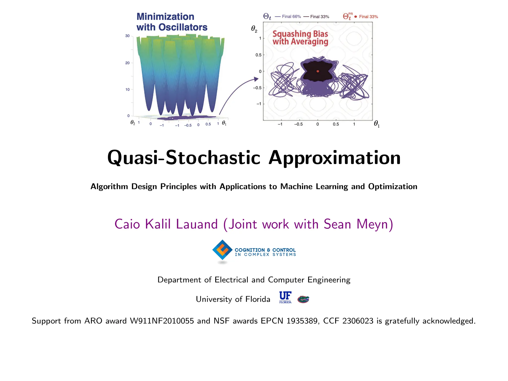
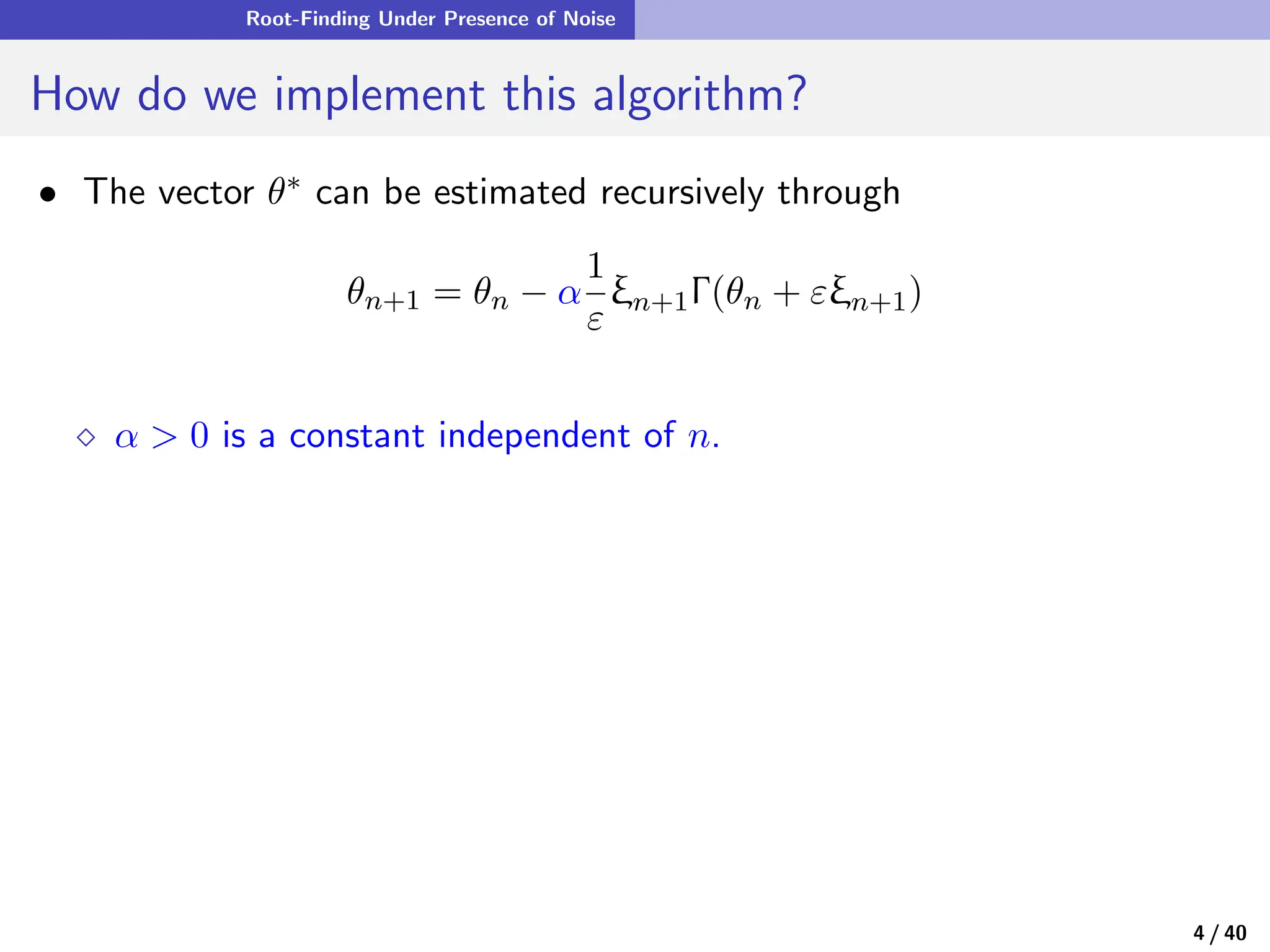
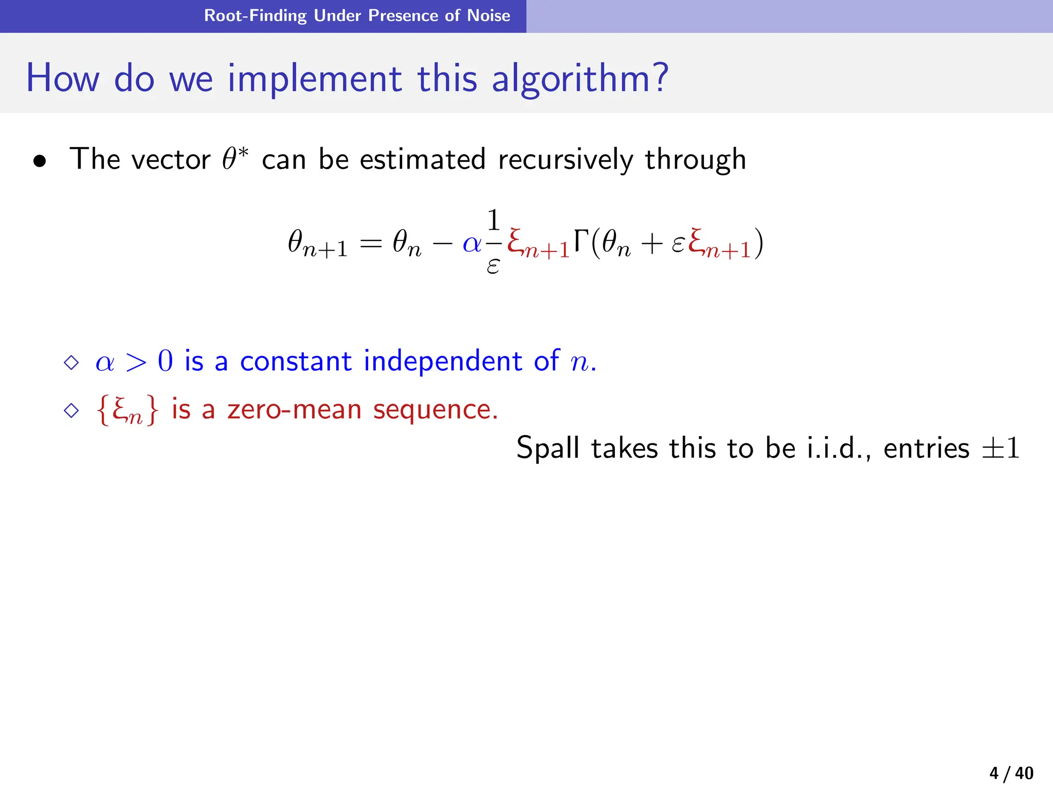
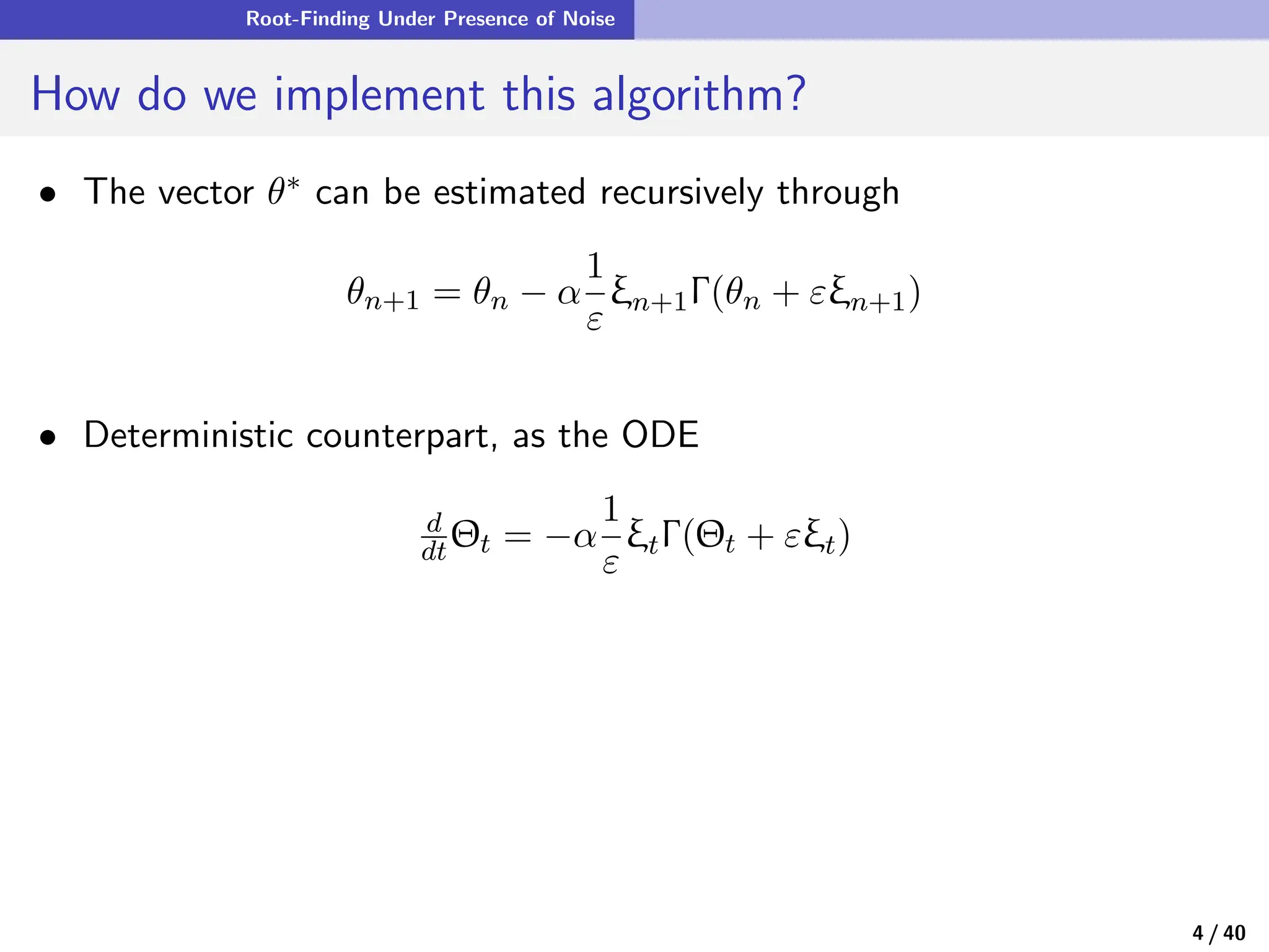
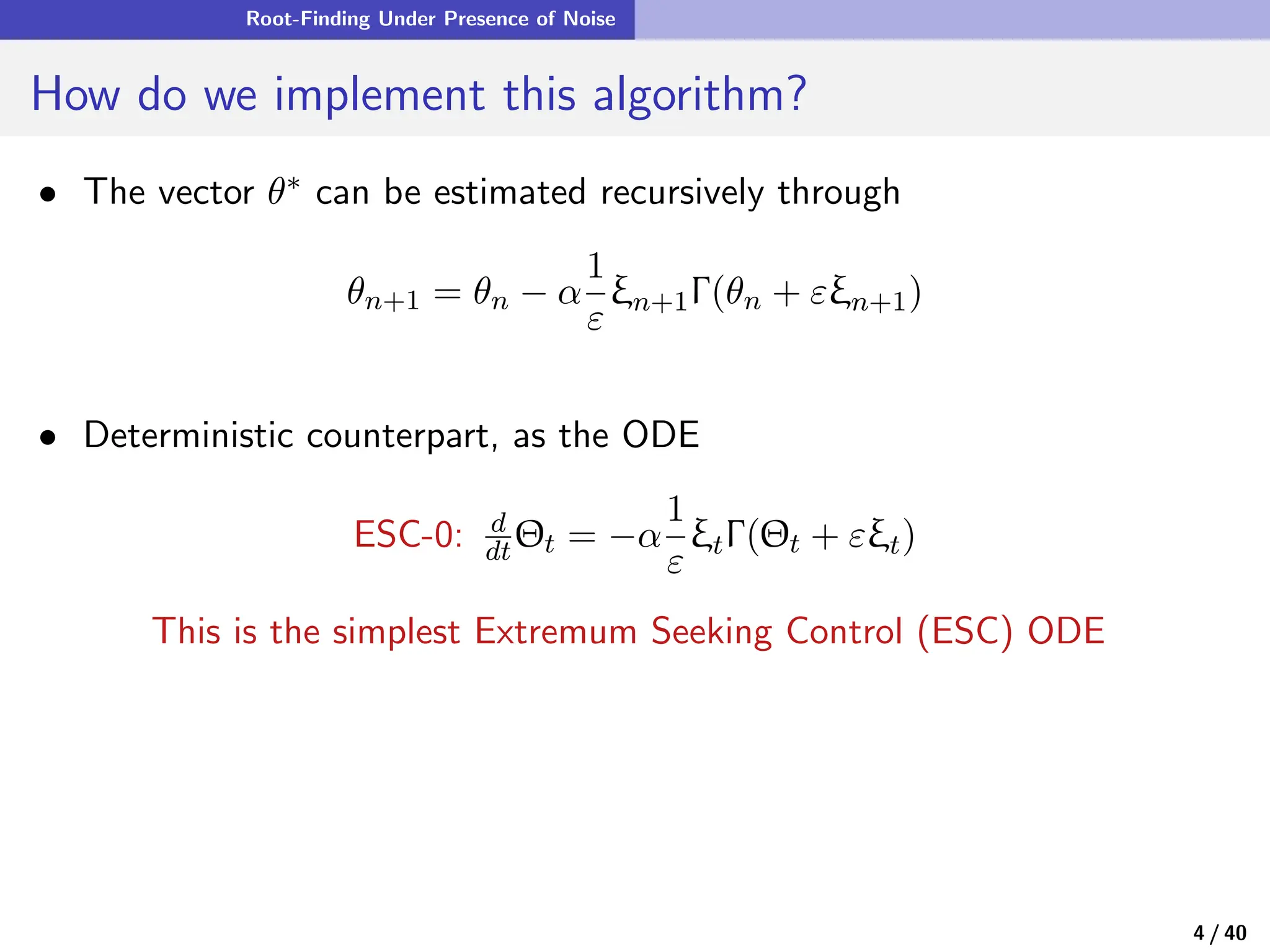
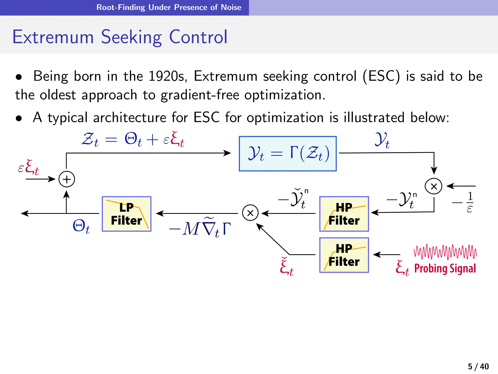
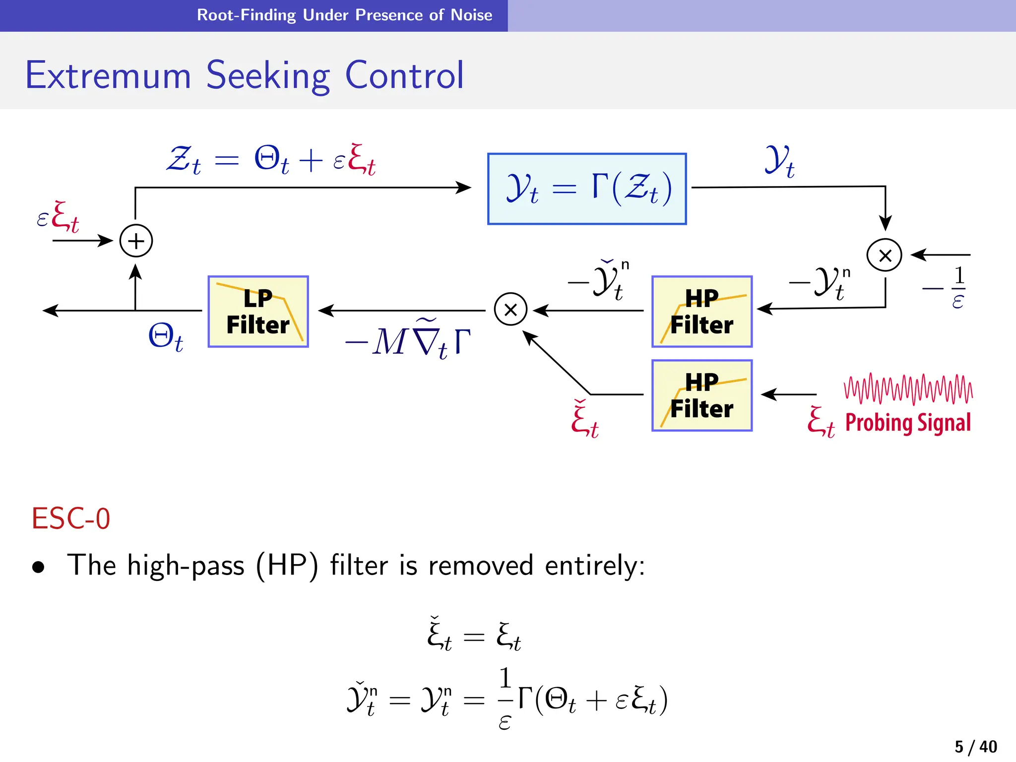
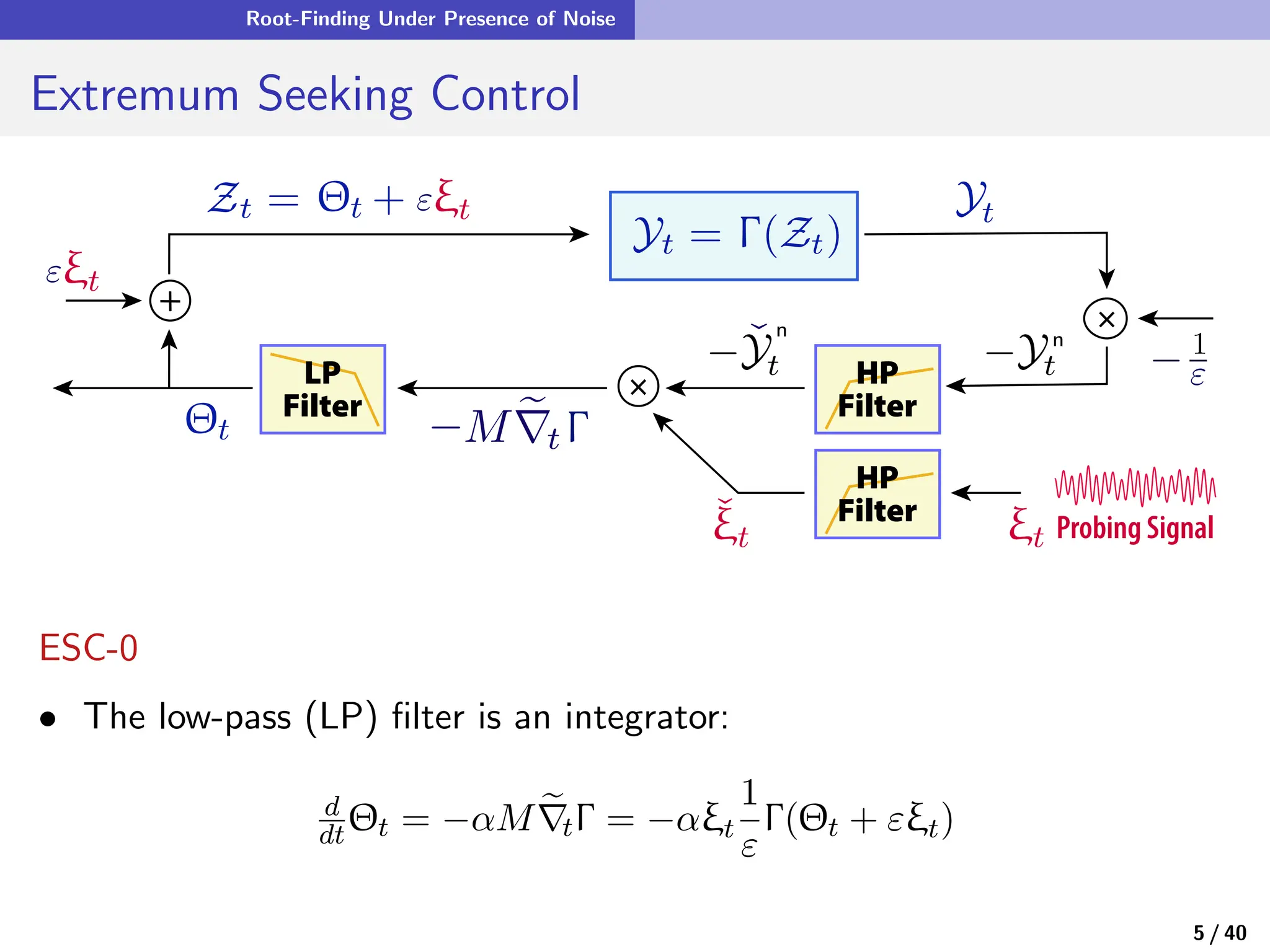
This document discusses the design principles of quasi-stochastic approximation algorithms, particularly in the context of machine learning and optimization. It covers challenges in root-finding and optimization under noise, the implementation of gradient-free optimization techniques, and the application of extremum seeking control. The document also introduces the concept of perturbative mean flow for enhancing algorithm stability and effectiveness.