Regression analysis

1. Regression Analysis
Md. Moyen Uddin PK

2. Why Regression Analysis ?
 Regression analysis is used;
 to understand which among the independent variables are related to the
dependent variable, and
 to explore the forms of these relationships.
 In restricted circumstances, regression analysis can be used to infer causal
relationships between the independent and dependent variables.

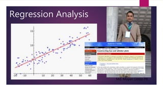
3. Simple Linear Regression Model
Yi=βo+β1Xi
Y=Dependent variable
βo=Constant, Y-axis intercept
β1= slope
X=independent variable
Xi
(Ethanol)
Yi
(% Yield)
100 % 26.12
80 % 22.45
70 % 18.67
60 % 14.56
50 % 11.23
40 % 9.61
y = 0.298x - 2.7893
R² = 0.974
0
5
10
15
20
25
30
0 20 40 60 80 100 120
%Yield
% Ethanol
Effect of solvents on % Yield Y=0.298X-2.7893
βo
β1
DV IV

4. Multiple Regression Model

5. SPSS analysis

6. Coefficients analysis….
The B coefficients tell us how many units BMI increases for a single unit increase in
each predictor.
Here, 1 point increase on the body weight corresponds to 0.366 points increase on
the BMI. We can predict BMI by computing;
BMI=52.899+(0.366*weight)+(0.333*height)+(0.00*Wc)+(0.020*Hc)+(0.003*Physical exercise)
The beta coefficients allow us to compare the
relative strengths of our predictors.
Y= β0+ β1X1+ β2X2+ β3X3+ β4X4+ β5X5
The standard errors are the standard deviations of our
coefficients over (hypothetical) repeated samples.
Smaller standard errors indicate more accurate
estimates

7. Model Summary…
R denotes the correlation between predicted and
observed BMI. In our case, R = 0.993. Since this is a very
high correlation, our model predicts BMI rather precisely.
R square is simply the square of R. It indicates the
proportion of variance in BMI that can be “explained” by
our FIVE predictors.
Because regression maximizes R
square for our sample, it will be somewhat
lower for the entire population, a
phenomenon known as shrinkage.
The adjusted R square estimates the
population R square for our model and thus
gives a more realistic indication of its
predictive power.

8. ANOVA Table analysis…