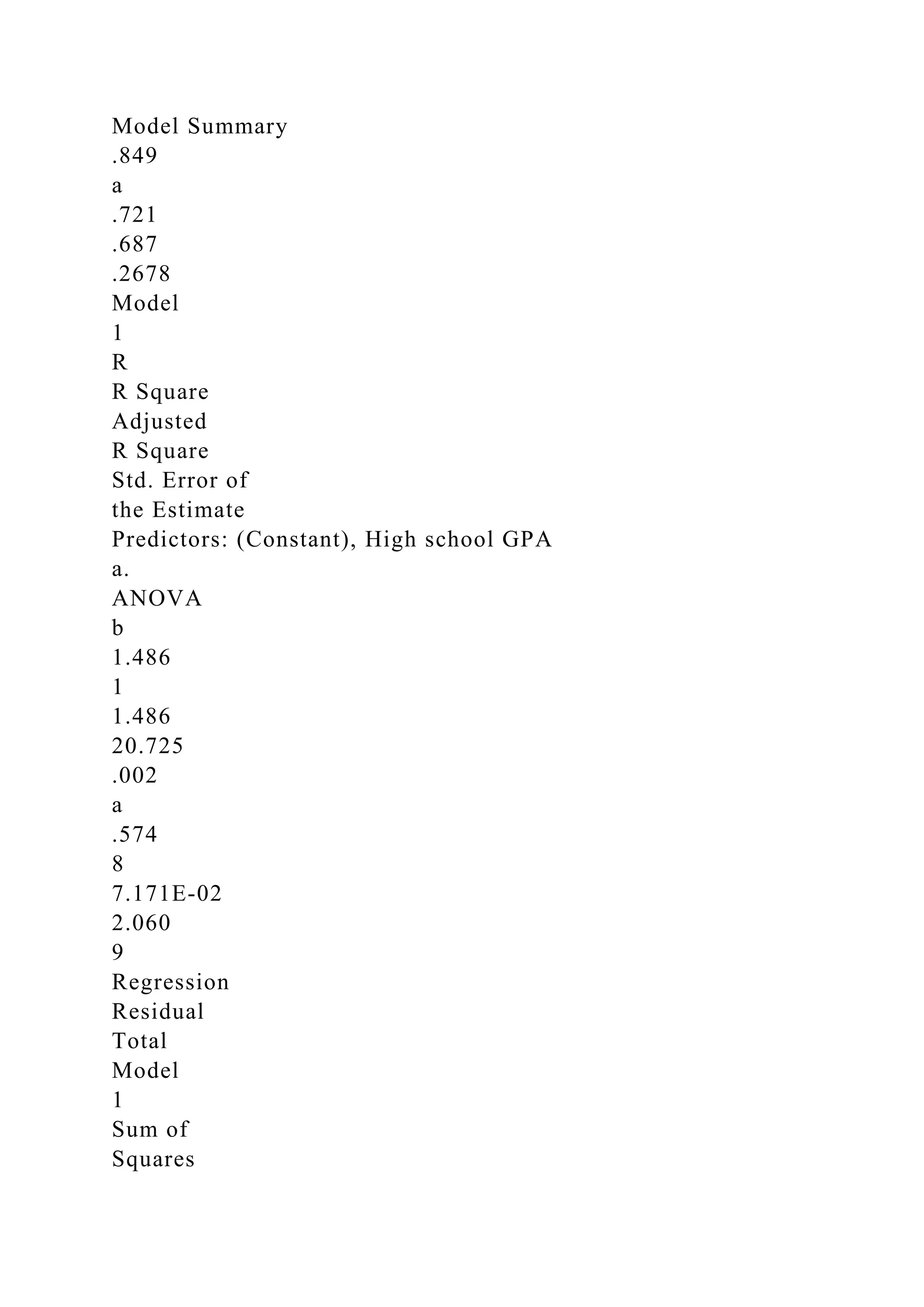
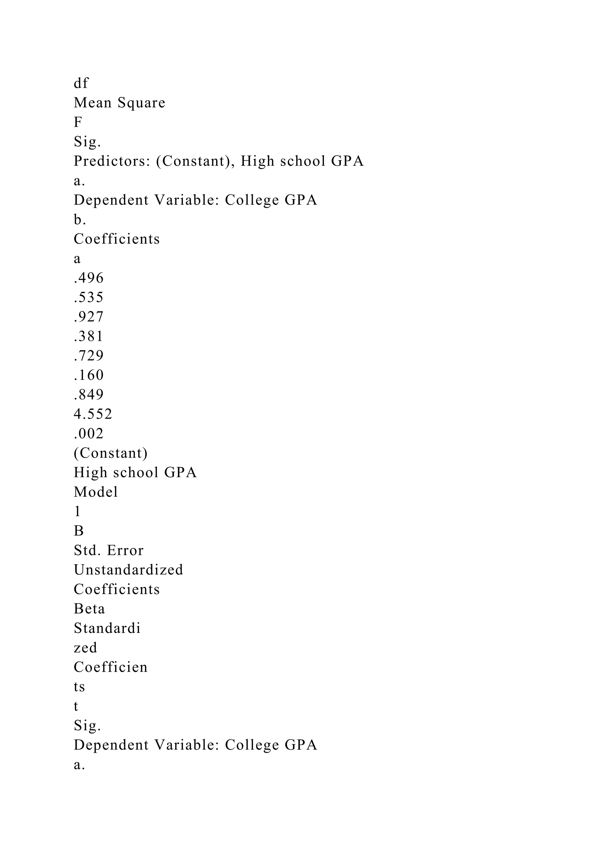
Correlation Analysis Correlation Analysis Correlation measures the relationship between two quantitative variables Linear correlation measures if the ordered paired data follow a straight-line relationship between quantitative variables. The correlation coefficient (r) computed from the sample data measures the strength and the direction of a linear relationship between two variables. The range of correlation coefficient is -1 to +1. When there is no linear relationship between the two variables or only a weak relationship, the value of correlation coefficient will be close to 0. Things to Remember Correlation coefficient cutoff points +0.30 to + 0.49 weak positive association. + 0.5 to +0.69 medium positive association. +0.7to + 1.0 strong positive association. - 0.5 to - 0.69 medium negative association. - 0.7 to - 1.0 strong negative association. - 0.30 to - 0.49 weak negative association. 0 to - 0.29 little or no association. 0 to + 0.29 little or no association. Relationships of Linear Correlation As x increases, no definite shift in y: no correlation. As x increase, a definite shift in y: correlation. Positive correlation: x increases, y increases. Negative correlation: x increases, y decreases. If the points exhibit some other nonlinear pattern: no linear relationship. Example: No correlation. As x increases, there is no definite shift in y. Example: Positive/direct correlation. As x increases, y also increases. Example: Negative/indirect/inverse correlation. As x increases, y decreases. Coefficient of linear correlation: r, measures the strength of the linear relationship between two variables. Pearson Correlation formula: Note: r = +1: perfect positive correlation r = -1 : perfect negative correlation Use the calculated value of the coefficient of linear correlation, r, to make an inference about the population correlation coefficient r. Example 1: Is there a relationship between age of the children and their score on the Child Medical Fear Scale (CMFS), using the data shown in Table 1? H0: There is no significant relationship between the age of the children and their score on the CMFS Or H0: r = 0 IDAge (x)CMFS (y)183129253940410275113569297825893498441011191172812647136421483715935161216171512181323191026201036 Table 1 Scattergram (Scatterplot) Age (x) = Independent variable, CMFS (y)= Dependent variable Correlation Coefficient The Results: a. Decision: Reject H0. b. Conclusion: There is evidence to suggest that there is a significant linear relationship between the age of the child and the score on the CMFS. Answers the question of whether there is a significant linear relationship or not Simple Linear Regression Analysis Linear Regression Analysis Linear Regression analysis finds the equation of the line that predicts the dependent variable based on the independent variable. 210 190 165 150 130 115 100 90 70 60 40 25 35 6.

1. Correlation Analysis
Correlation Analysis
Correlation measures the relationship between two quantitative
variables
Linear correlation measures if the ordered paired data follow a
straight-line relationship between quantitative variables.
The correlation coefficient (r) computed from the sample data
measures the strength and the direction of a linear relationship
between two variables.
The range of correlation coefficient is -1 to +1. When there is
no linear relationship between the two variables or only a weak
relationship, the value of correlation coefficient will be close to
0.
Things to Remember
Correlation coefficient cutoff points
+0.30 to + 0.49 weak positive association.
+ 0.5 to +0.69 medium positive association.

2. +0.7to + 1.0 strong positive association.
- 0.5 to - 0.69 medium negative association.
- 0.7 to - 1.0 strong negative association.
- 0.30 to - 0.49 weak negative association.
0 to - 0.29 little or no association.
0 to + 0.29 little or no association.
Relationships of Linear Correlation
As x increases, no definite shift in y: no correlation.
As x increase, a definite shift in y: correlation.
Positive correlation: x increases, y increases.
Negative correlation: x increases, y decreases.
If the points exhibit some other nonlinear pattern: no linear
relationship.

3. Example: No correlation.
As x increases, there is no definite shift in y.
Example: Positive/direct correlation.
As x increases, y also increases.
Example: Negative/indirect/inverse correlation.
As x increases, y decreases.
Coefficient of linear correlation: r, measures the strength of the
linear relationship between two variables.
Pearson Correlation formula:
Note:
r = +1: perfect positive correlation
r = -1 : perfect negative correlation
Use the calculated value of the coefficient of linear correlation,
r, to make an inference about the population correlation
coefficient r.

4. Example 1: Is there a relationship between age of the children
and their score on the Child Medical Fear Scale (CMFS), using
the data shown in Table 1?
H0: There is no significant relationship between the age of the
children and their score on the CMFS
Or
H0: r = 0
IDAge (x)CMFS
(y)18312925394041027511356929782589349844101119117281
2647136421483715935161216171512181323191026201036
Table 1
Scattergram (Scatterplot)
Age (x) = Independent variable, CMFS (y)= Dependent variable

5. Correlation Coefficient
The Results:
a. Decision: Reject H0.
b. Conclusion: There is evidence to suggest that there is a
significant linear relationship between the age of the child and
the score on the CMFS.
Answers the question of whether there is a significant linear
relationship or not
Simple Linear Regression Analysis
Linear Regression Analysis
Linear Regression analysis finds the equation of the line that
predicts the dependent variable based on the independent
variable.
210 190 165 150 130 115 100 90 70 60 40 25 35
60 75 85 100 110 120 130 140 150
Drug A (dose in mg)
Symptom Index
210 190 165 150 130 115 100 90 70 60 40 25 35
60 75 85 100 110 120 130 140 150
Drug A (dose in mg)

6. Symptom Index
y = dependent (predicted )variable
a = y intercept (constant)
b = slope (regression coefficient) of line
x = independent (predictor) variable
y = a + bx
Y
X
Simple Linear Regression Assumptions:
Normality
Equal variances
Independence
Linear relationship
Regression analysis establishes a regression equation for
predictions
For a given value of x, we can predict a value of y
How good is the predictor?
Very good predictor
Moderate predictor
210 190 165 150 130 115 100 90 70 60 40 25 35
60 75 85 100 110 120 130 140 150

7. Drug A (dose in mg)
Symptom Index
210 190 165 150 130 115 100 90 70 60 40 50 30
60 80 60 110 90 140 110 140 130
Drug B (dose in mg)
Symptom Index
How good is the predictor? R2
For simple regression, Coefficient of determination (R2) is the
square of the correlation coefficient
Reflects variance accounted for in data by the best-fit line
Takes values between 0 (0%) and 1 (100%)
Frequently expressed as percentage, rather than decimal
Coefficient of Determination (R2)
High variance explained
Less variance explained
210 190 165 150 130 115 100 90 70 60 40 25 35
60 75 85 100 110 120 130 140 150
Drug A (dose in mg)
Symptom Index
210 190 165 150 130 115 100 90 70 60 40 50 30
60 80 60 110 90 140 110 140 130

8. Drug B (dose in mg)
Symptom Index
Previous example: Scatter gram (Scatterplot)
Age (x) = Independent variable, CMFS (y)= Dependent variable
95% Confidence Interval
Regression Line
Correlation Coefficient
Coefficient of Determination (R2)
(Gives the % of variation)
Example 2: A recent article measured the job satisfaction of
subjects. The data below represents the job satisfaction scores,
y, and the salaries (in thousands), x, for a sample of similar
individuals.

9. 1. Draw a scatter diagram for this data.
2. Find the equation of the line of best fit.
IDSalaries (x)Scores
(y)1311723320322134241553518629177231283721
Scatter gram:
The Regression Equation:
Thus a salary of $30,000 will result in a score of 17.
Example 3: Is high school GPA a useful predictor of college
GPA, using the data shown in Table 2?IDHS GPACollege
GPA14.003.8023.702.7032.202.3043.803.2053.803.5062.802.40
73.002.6083.403.0093.302.70103.002.80
Table 2:
Scattergram:

10. Results:
Correlation Analysis
There is a significant linear relationship between high school
GPA and College GPA.
Regression Analysis
72.1% of the variation in college GPA is explained by high
school GPA
Regression equation: College GPA = 0.50 + 0.73 HS GPA
Conclusion: High school GPA is a useful predictor of college
GPA
3
0
2
0
1
0
5
5
4
5
3
5
I
n
p
u
t
O
u
t
p
u
t
5

11. 5
5
0
4
5
4
0
3
5
3
0
2
5
2
0
1
5
1
0
6
0
5
0
4
0
3
0
2
0
I
n
p
u
t
O
u

12. t
p
u
t
5
5
5
0
4
5
4
0
3
5
3
0
2
5
2
0
1
5
1
0
9
5
8
5
7
5
6
5
5
5
I
n

13. p
u
t
O
u
t
p
u
t
r
x
x
y
y
n
s
s
x
y
=
-
-
-
å
(
)(
)
(
)
1
11
r
-££+
Model Summary
.748
a

14. .560
.535
6.3442
Model
1
R
R Square
Adjusted
R Square
Std. Error of
the Estimate
Predictors: (Constant), Age
a.
0
20
40
60
80
100
120
140
160
180
200
050100150200250
1.49.517()
1.49.517(30)
Scoresalaries
Score
=+
=+
Coefficients
a
1.490
2.327
.640

15. .546
.517
.078
.938
6.613
.001
(Constant)
SALARIES
Model
1
B
Std. Error
Unstandardized
Coefficients
Beta
Standardi
zed
Coefficien
ts
t
Sig.
Dependent Variable: Job Satisfaction
a.
High school GPA
4.54.03.53.02.52.0
College GPA
4.0
3.8
3.6
3.4
3.2
3.0
2.8
2.6
2.4
2.2

16. Model Summary
.849
a
.721
.687
.2678
Model
1
R
R Square
Adjusted
R Square
Std. Error of
the Estimate
Predictors: (Constant), High school GPA
a.
ANOVA
b
1.486
1
1.486
20.725
.002
a
.574
8
7.171E-02
2.060
9
Regression
Residual
Total
Model
1
Sum of
Squares

17. df
Mean Square
F
Sig.
Predictors: (Constant), High school GPA
a.
Dependent Variable: College GPA
b.
Coefficients
a
.496
.535
.927
.381
.729
.160
.849
4.552
.002
(Constant)
High school GPA
Model
1
B
Std. Error
Unstandardized
Coefficients
Beta
Standardi
zed
Coefficien
ts
t
Sig.
Dependent Variable: College GPA
a.