This document provides an introduction to correlation and regression. It defines correlation as a measure of the association between two numerical variables, and describes positive and negative correlation. Regression analysis is introduced as a method to describe and predict the relationship between two variables. The key aspects of simple linear regression are discussed, including determining the line of best fit and evaluating the model performance using the coefficient of determination (R2).
Introduction and overview of correlation and regression topics by S.V. Bhaskar, Associate Professor.
Definition of correlation as a measure of association between two numerical variables. Example of positive correlation with temperature and thirst, illustrated with a temperature vs water consumption graph.
Presentation of scatter plots to illustrate different types of correlations: positive, negative, and lack of correlation with visual examples.
Introduction to Pearson's correlation coefficient (r), measuring strength and direction of relationships, its range, and caveats regarding correlation not indicating causation.
Detailed discussion on interpreting the correlation coefficient values (r), differentiating strengths of associations from strong to weak.
Formulas and methods for computing the correlation coefficient r, including concepts of covariance, paired items, and standard deviations.
Introduction to regression analysis, focusing on describing the relationship between two variables, its applications for prediction and control.
Understanding simple linear regression, its assumptions, the population regression function vs sample regression function, and the equation of regression lines.
Steps to obtain a regression solution from scatterplot visualization to calculating regression equations, along with example data.
Discussion of goodness of fit using R² to explain variability in dependent variables, with examples of temperature affecting water consumption.
Insights into interpreting regression outputs, including coefficients, slope, and y-intercept with real-world application perspectives.
Understanding null and alternative hypotheses in regression, significance testing, p-values, and criteria for rejecting the null hypothesis.
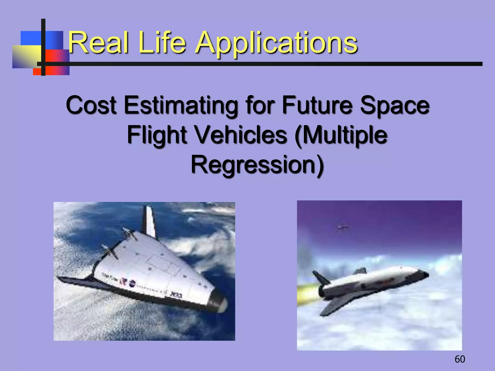
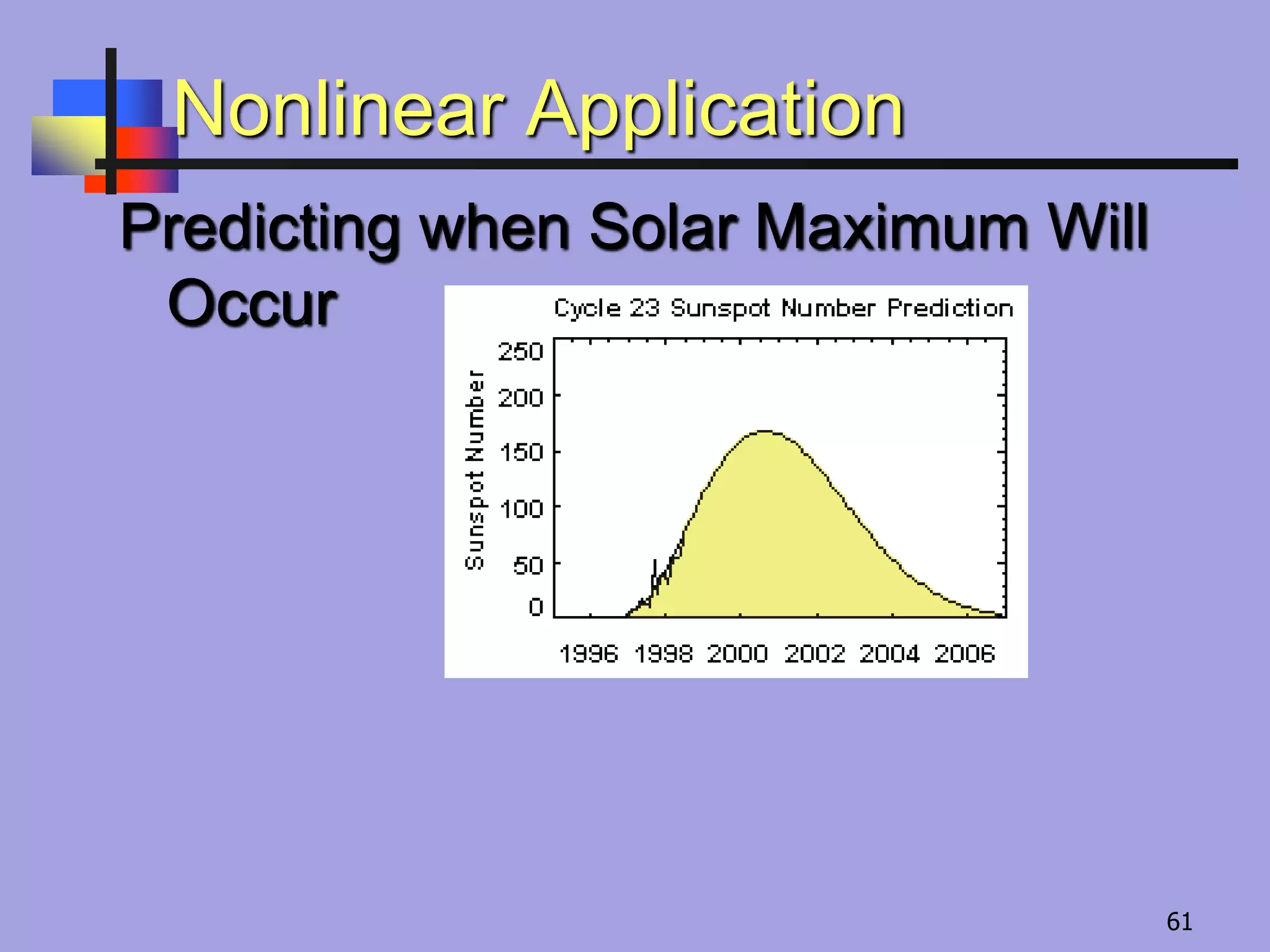
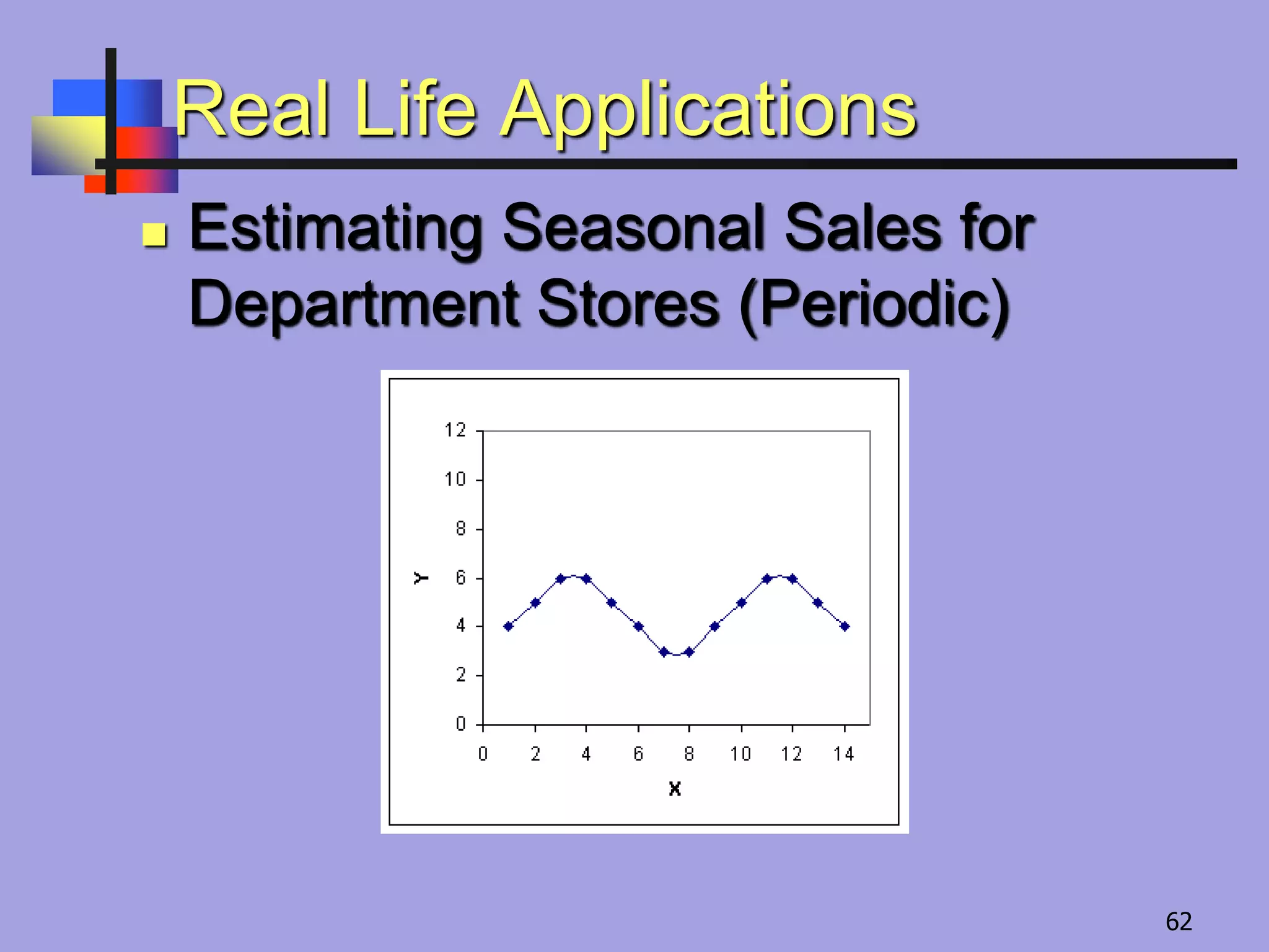
Examples of real-life applications including cost estimation for space vehicles, predicting solar maximum occurrences, and seasonal sales estimation.
Closure of the presentation thanking the audience.
Introduction to
Correlation andRegression
.S.V. Bhaskar,
Associate Professor,
Department of Mechanical Engineering,
Sanjivani College of Engineering,
Kopargaon (MS), INDIA.
1
2.
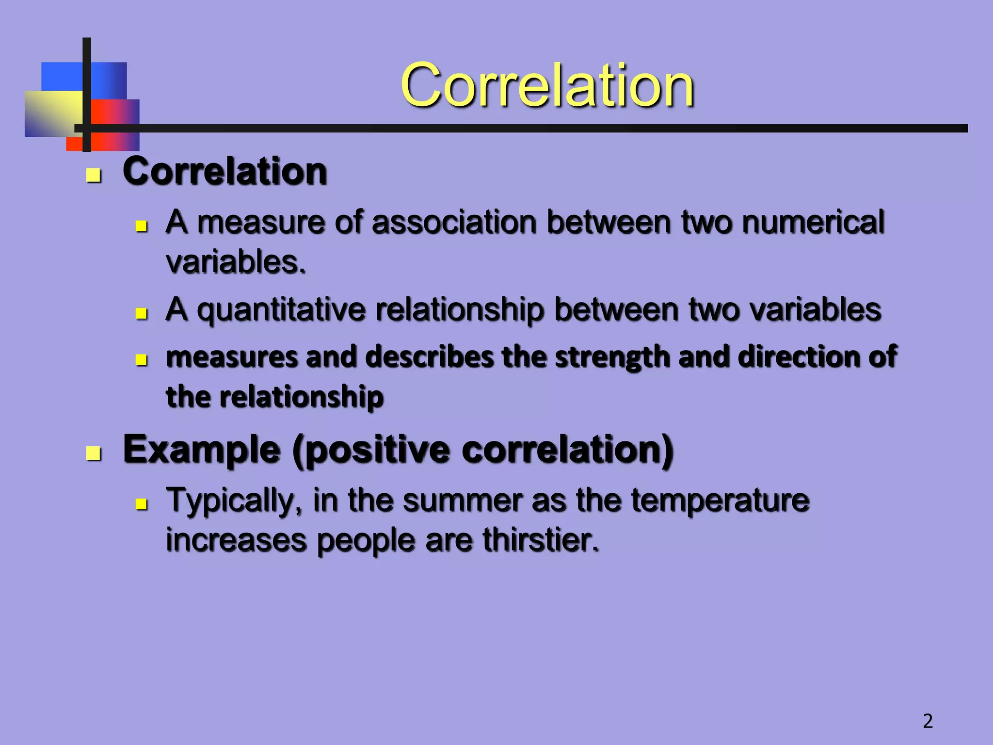
Correlation
Correlation
Ameasure of association between two numerical
variables.
A quantitative relationship between two variables
measures and describes the strength and direction of
the relationship
Example (positive correlation)
Typically, in the summer as the temperature
increases people are thirstier.
2
3.
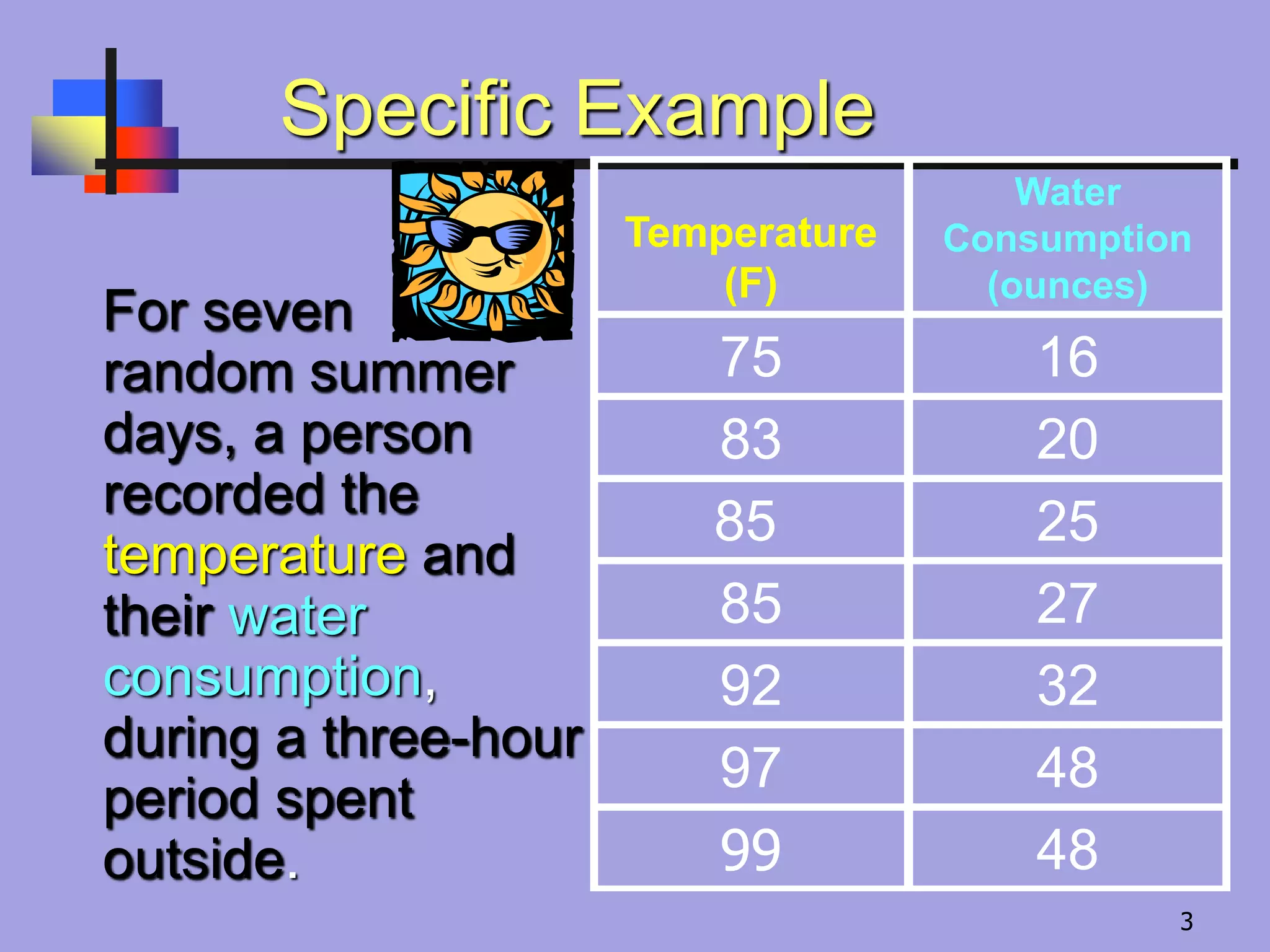
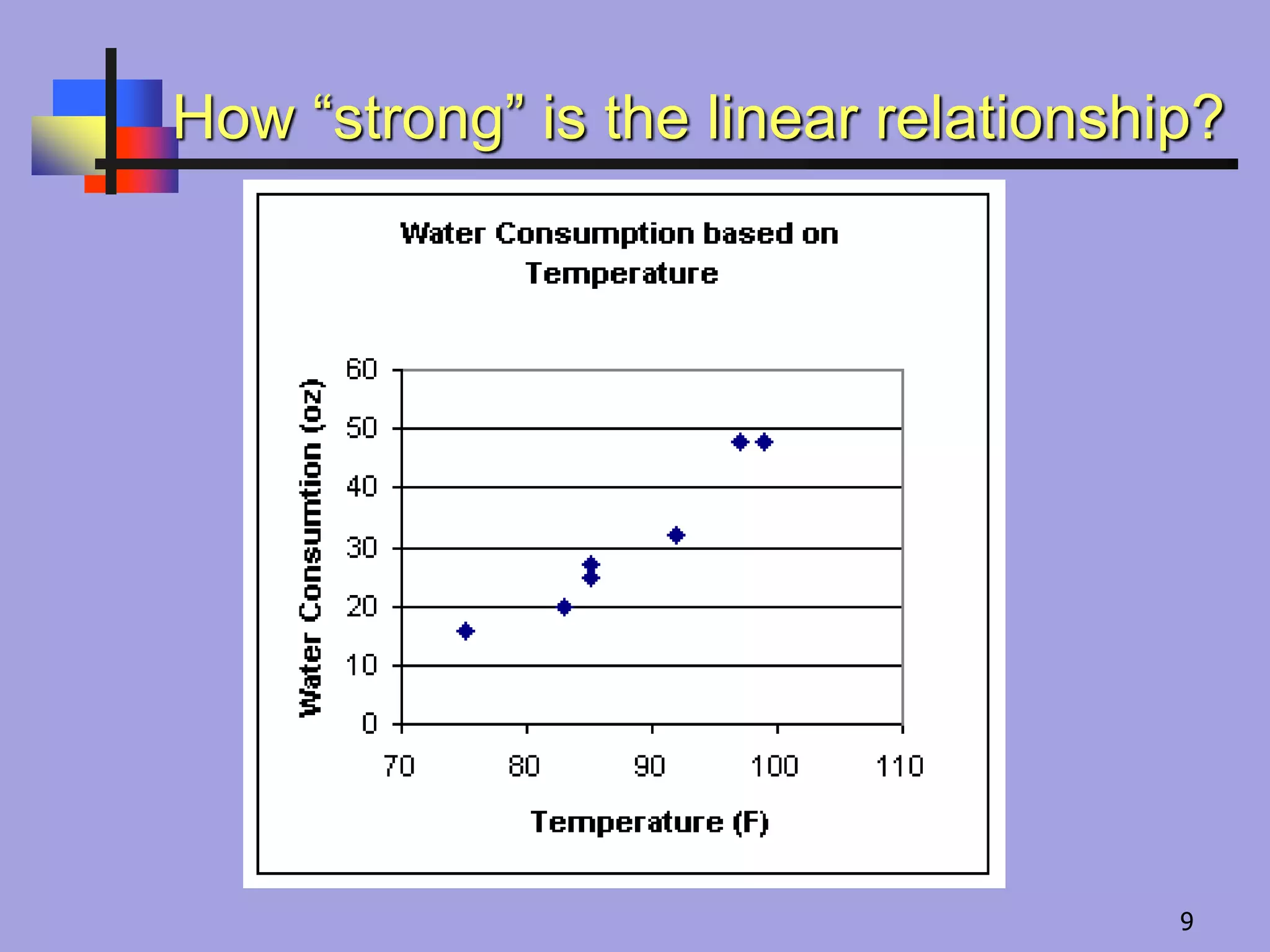
Specific Example
For seven
randomsummer
days, a person
recorded the
temperature and
their water
consumption,
during a three-hour
period spent
outside.
Temperature
(F)
Water
Consumption
(ounces)
75 16
83 20
85 25
85 27
92 32
97 48
99 48
3
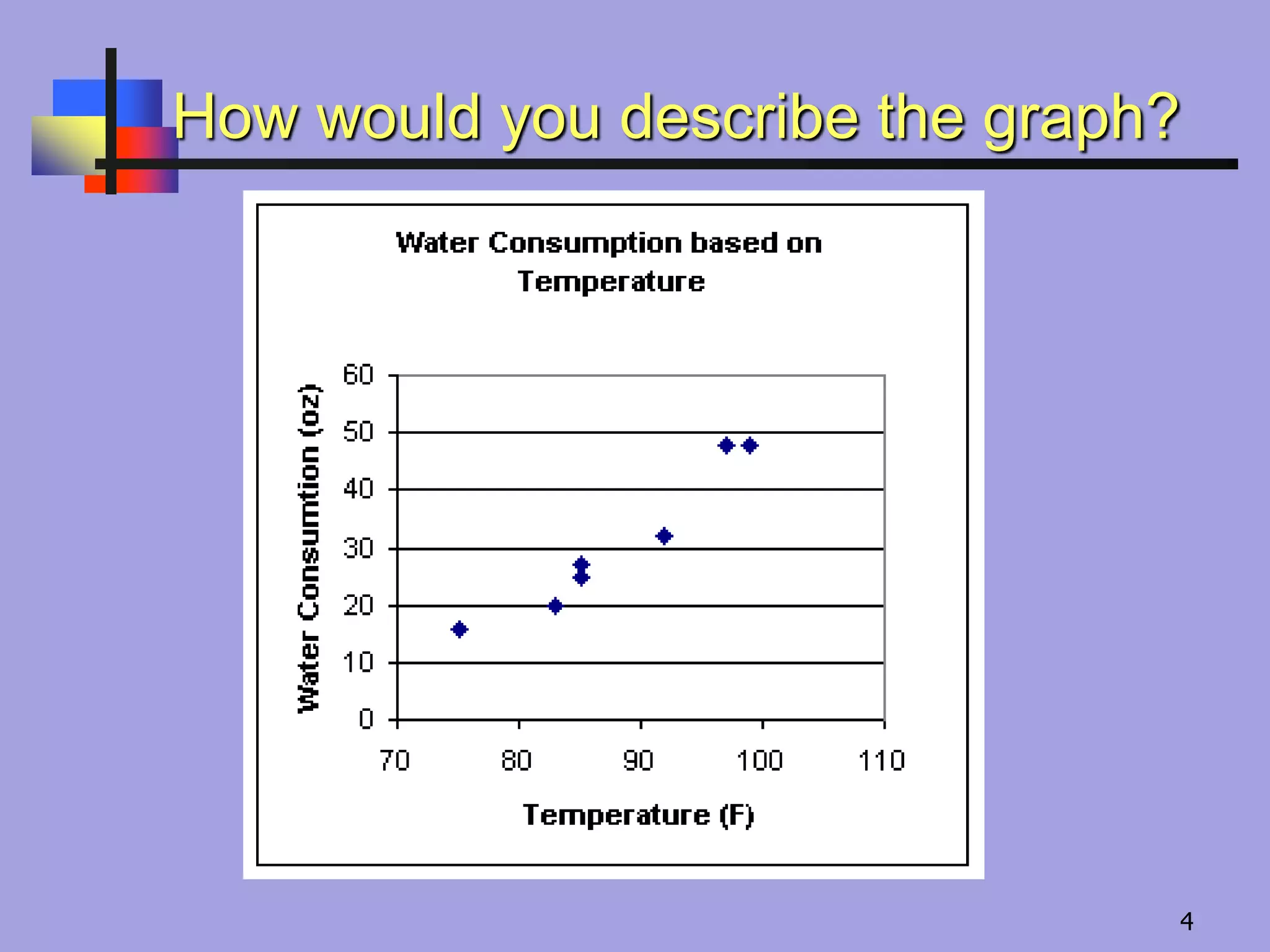
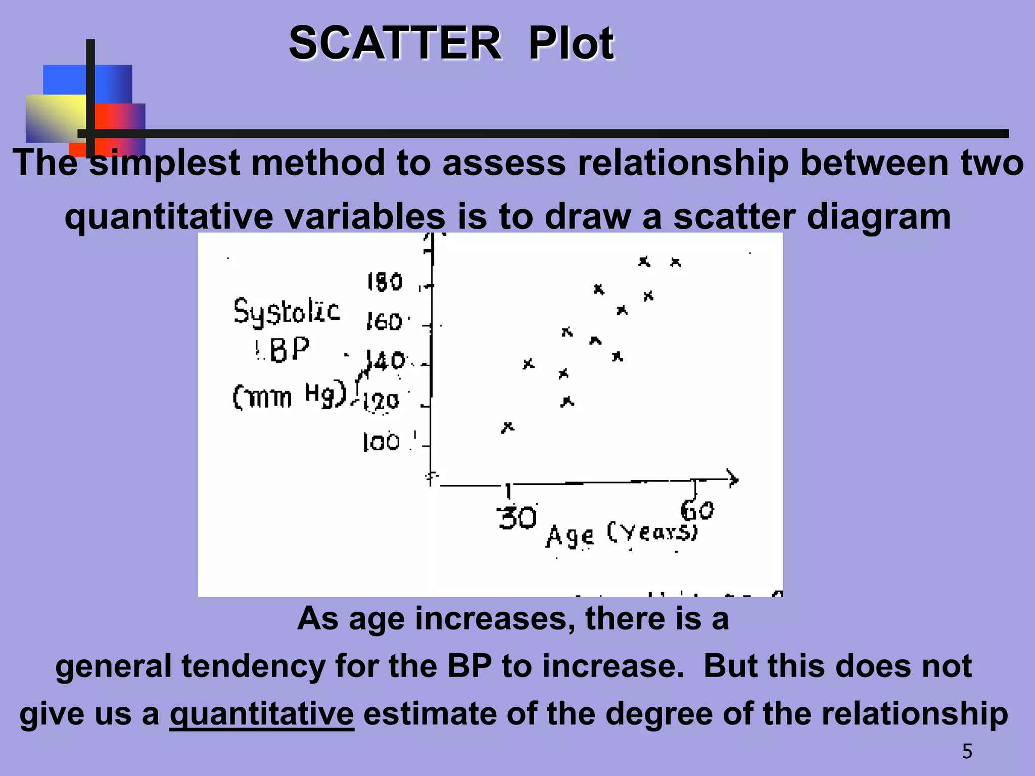
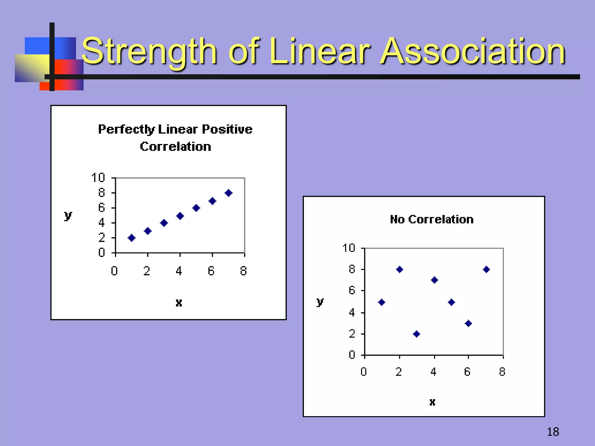
SCATTER Plot
The simplestmethod to assess relationship between two
quantitative variables is to draw a scatter diagram
As age increases, there is a
general tendency for the BP to increase. But this does not
give us a quantitative estimate of the degree of the relationship
5
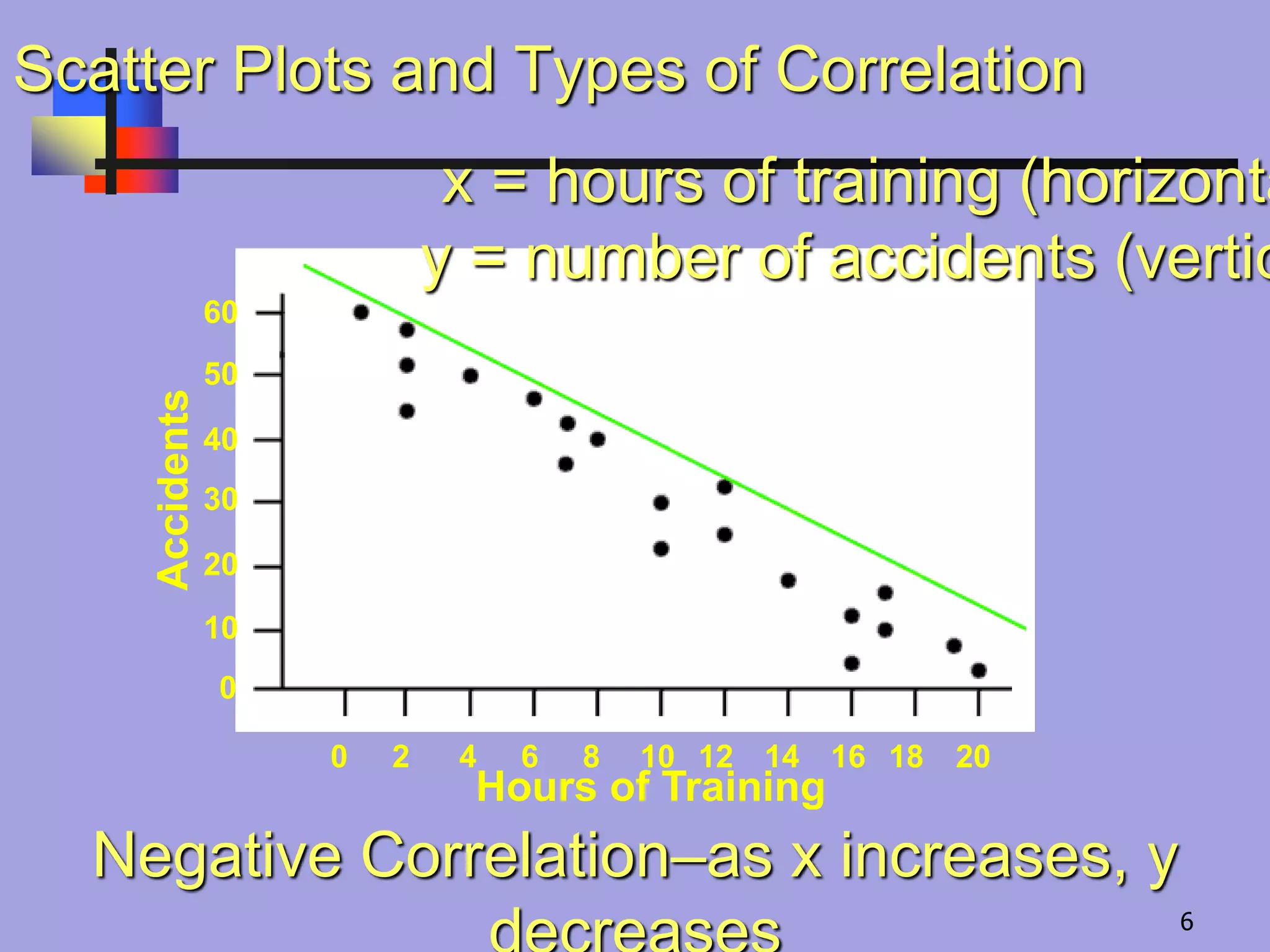
6.
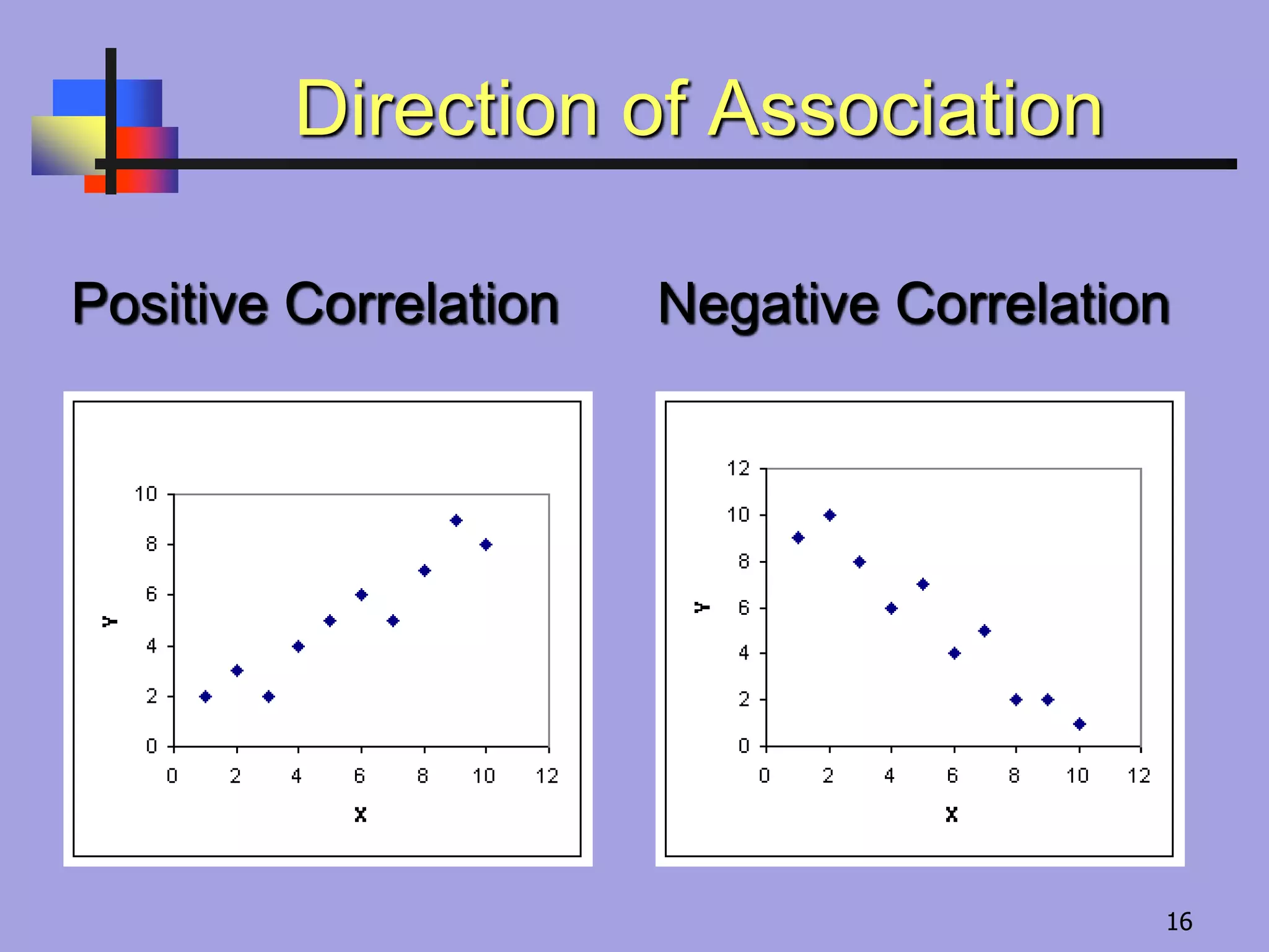
Negative Correlation–as xincreases, y
x = hours of training (horizonta
y = number of accidents (vertic
Scatter Plots and Types of Correlation
60
50
40
30
20
10
0
0 2 4 6 8 10 12 14 16 18 20
Hours of Training
Accidents
6
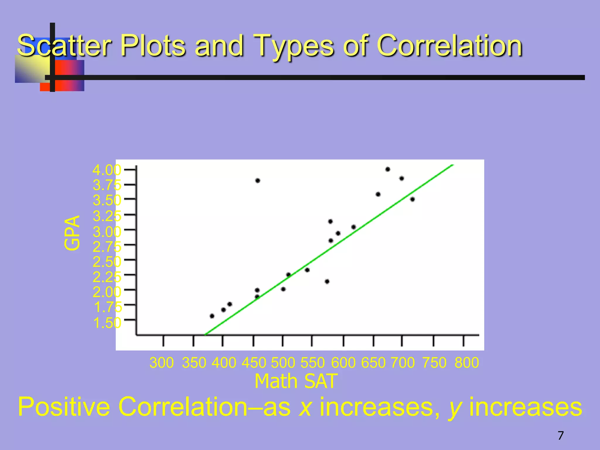
7.
Positive Correlation–as xincreases, y increases
GPA
Scatter Plots and Types of Correlation
4.00
3.75
3.50
3.00
2.75
2.50
2.25
2.00
1.50
1.75
3.25
300 350 400 450 500 550 600 650 700 750 800
Math SAT
7
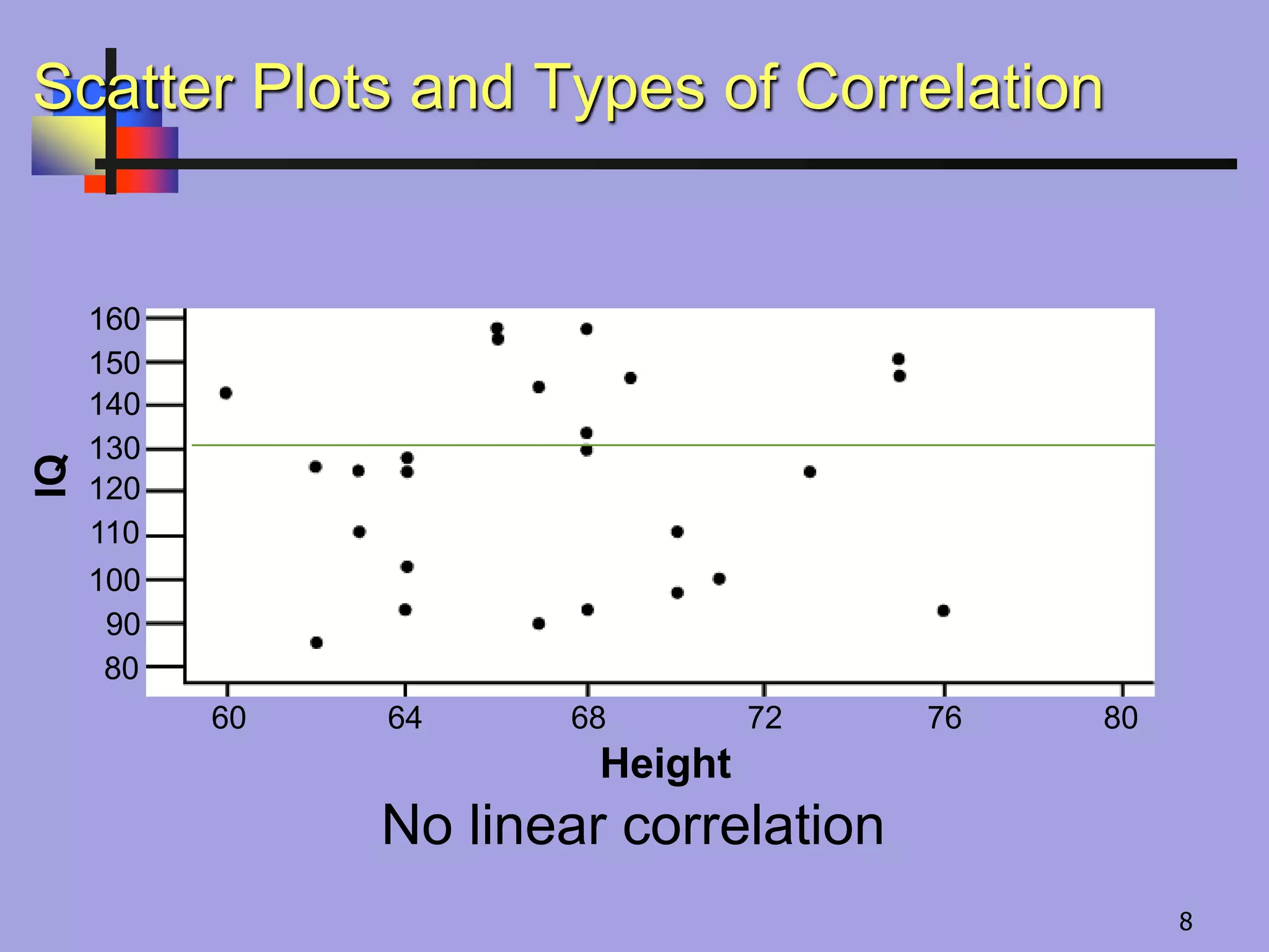
8.
No linear correlation
ScatterPlots and Types of Correlation
160
150
140
130
120
110
100
90
80
60 64 68 72 76 80
Height
IQ
8
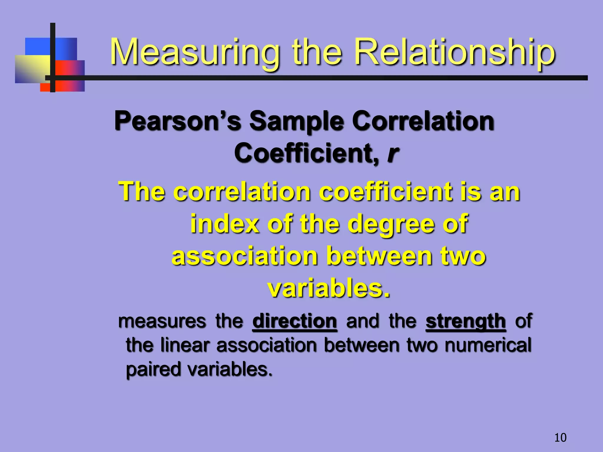
Measuring the Relationship
Pearson’sSample Correlation
Coefficient, r
The correlation coefficient is an
index of the degree of
association between two
variables.
measures the direction and the strength of
the linear association between two numerical
paired variables.
10
11.
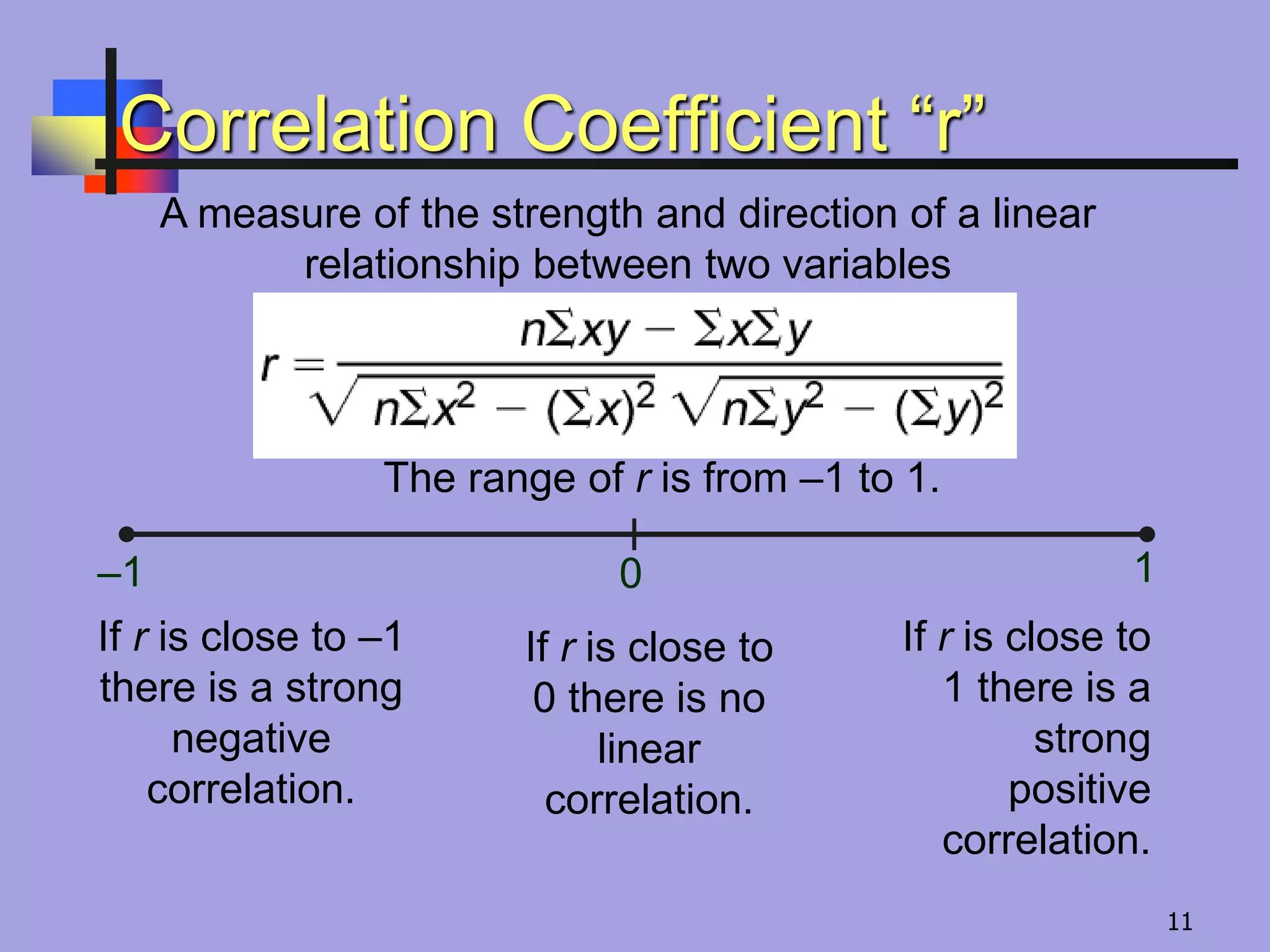
Correlation Coefficient “r”
Ameasure of the strength and direction of a linear
relationship between two variables
The range of r is from –1 to 1.
If r is close to
1 there is a
strong
positive
correlation.
If r is close to –1
there is a strong
negative
correlation.
If r is close to
0 there is no
linear
correlation.
–1 0 1
11
12.
High values ofone variable tend to occur with high
values of the other (and low with low)
In such situations, we say that there is a positive correlation
High values of one variable occur with low values of the other
(and vice-versa)
we say that there is a negative correlation
12
13.
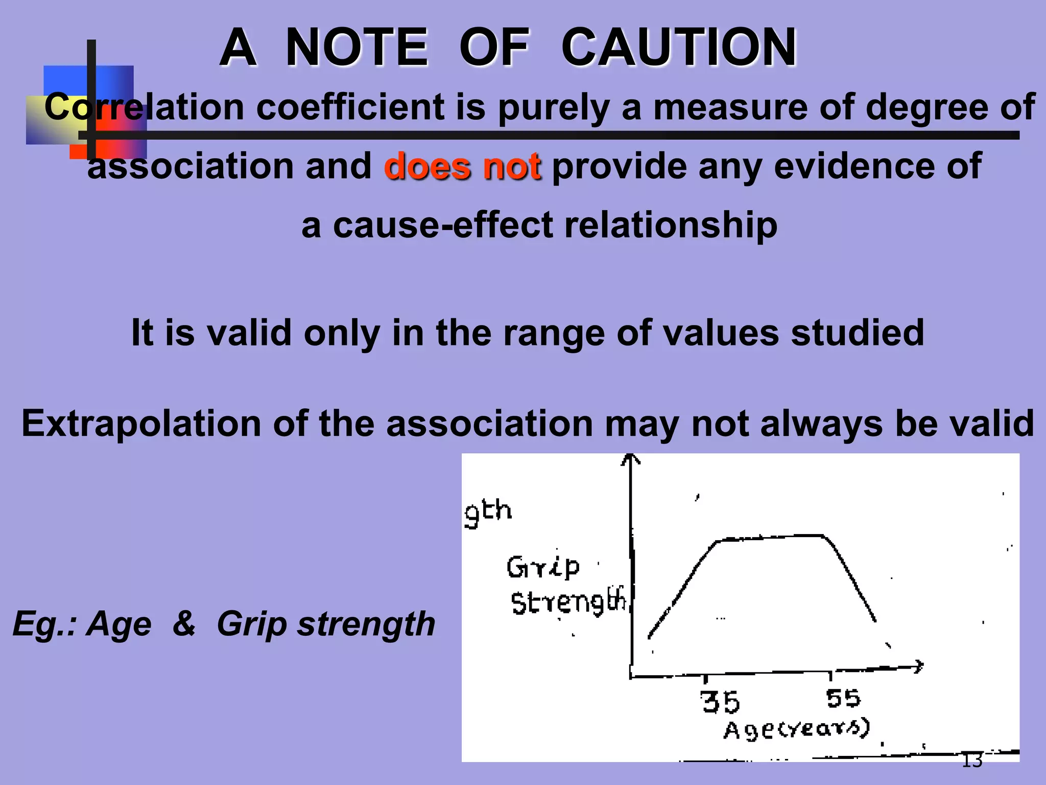
A NOTE OFCAUTION
Correlation coefficient is purely a measure of degree of
association and does not provide any evidence of
a cause-effect relationship
It is valid only in the range of values studied
Extrapolation of the association may not always be valid
Eg.: Age & Grip strength
13
14.
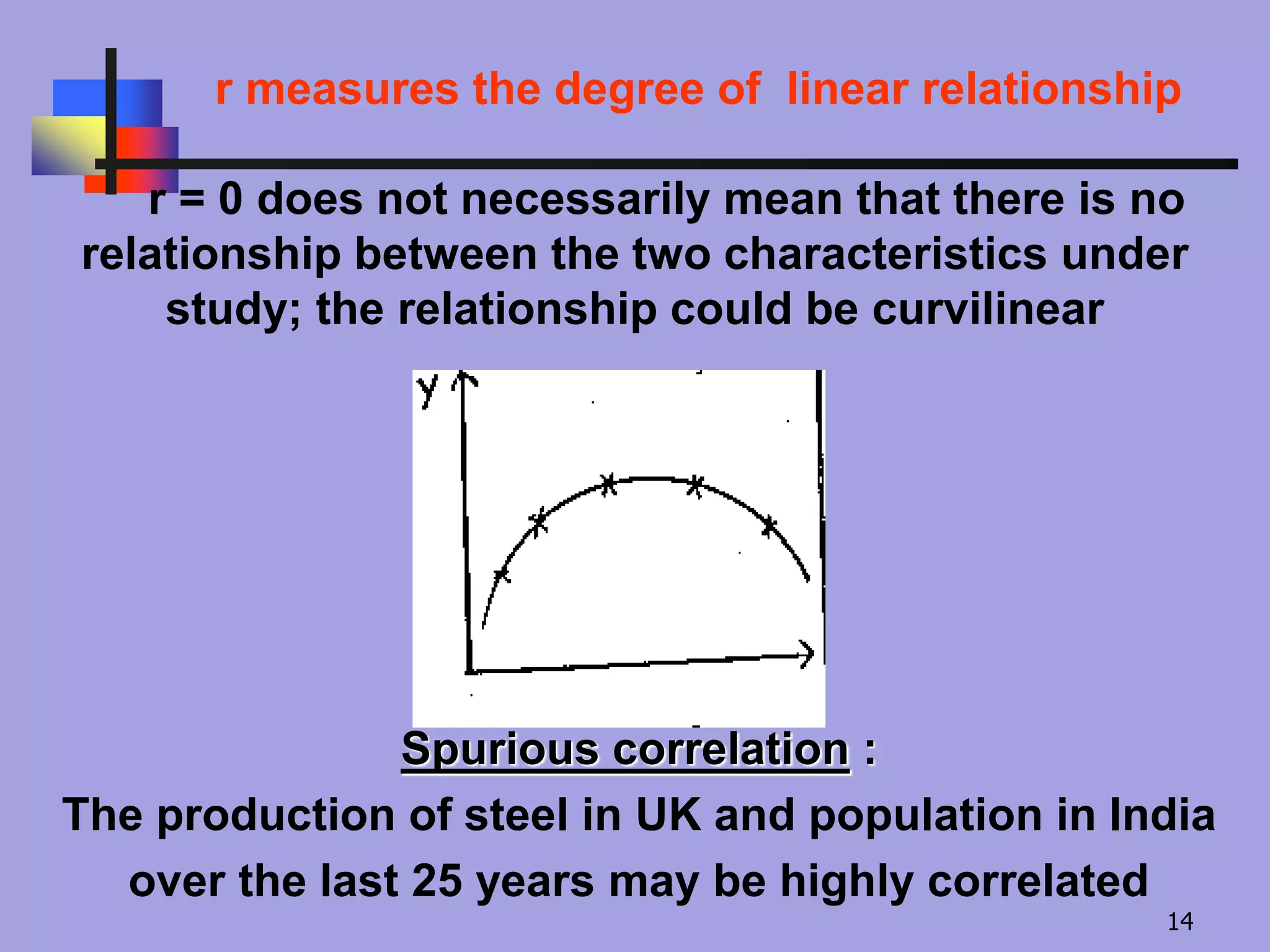
r measures thedegree of linear relationship
r = 0 does not necessarily mean that there is no
relationship between the two characteristics under
study; the relationship could be curvilinear
Spurious correlation :
The production of steel in UK and population in India
over the last 25 years may be highly correlated
14
15.
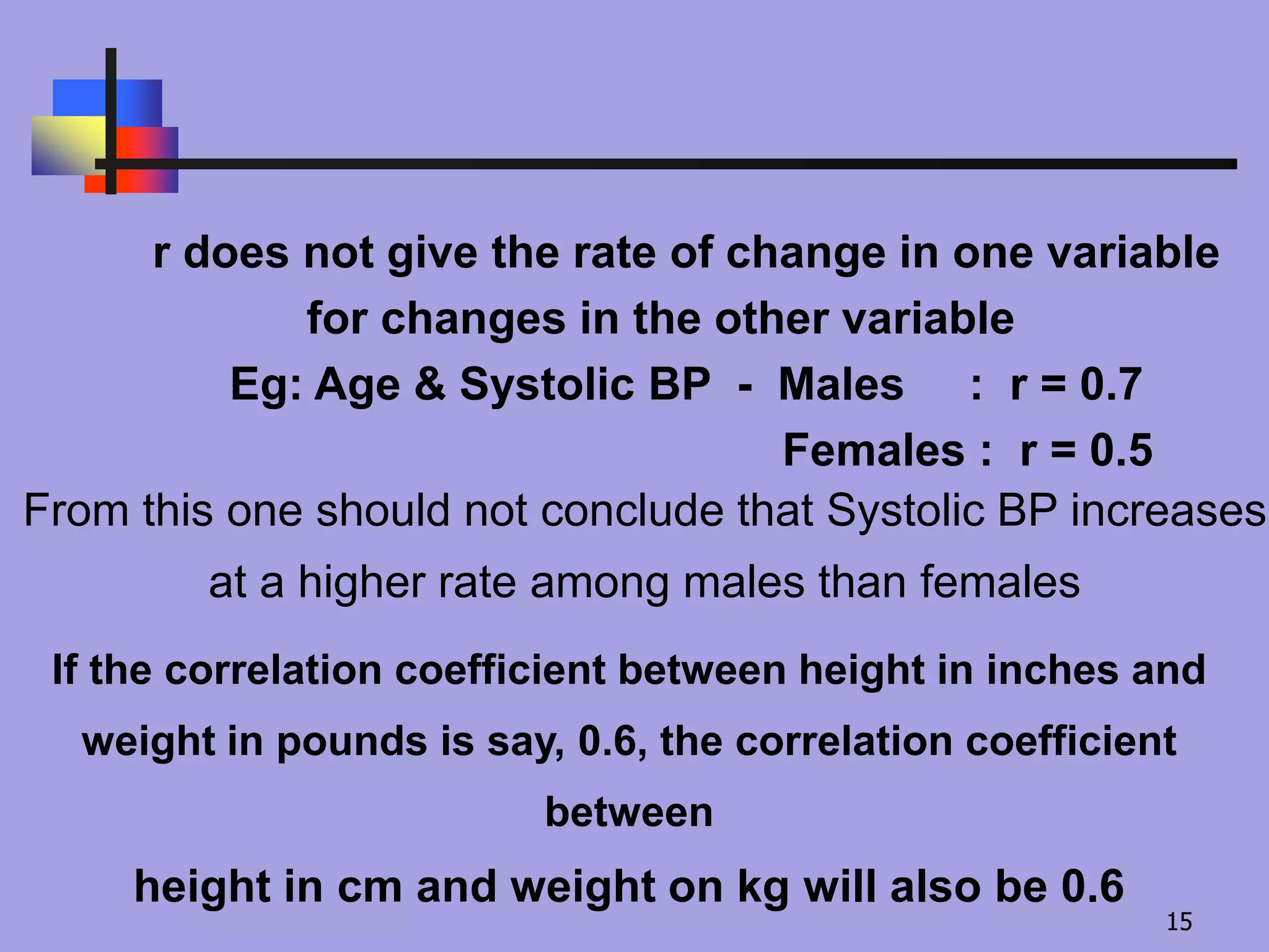
r does notgive the rate of change in one variable
for changes in the other variable
Eg: Age & Systolic BP - Males : r = 0.7
Females : r = 0.5
From this one should not conclude that Systolic BP increases
at a higher rate among males than females
If the correlation coefficient between height in inches and
weight in pounds is say, 0.6, the correlation coefficient
between
height in cm and weight on kg will also be 0.6
15
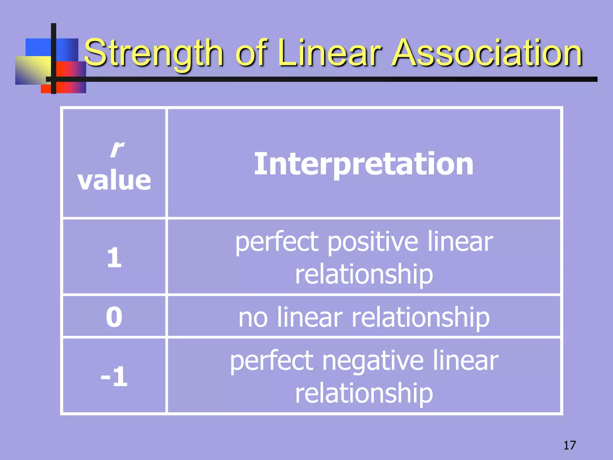
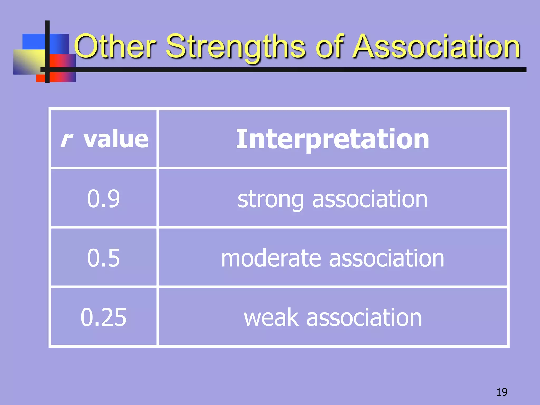
Strength of LinearAssociation
r
value
Interpretation
1
perfect positive linear
relationship
0 no linear relationship
-1
perfect negative linear
relationship
17
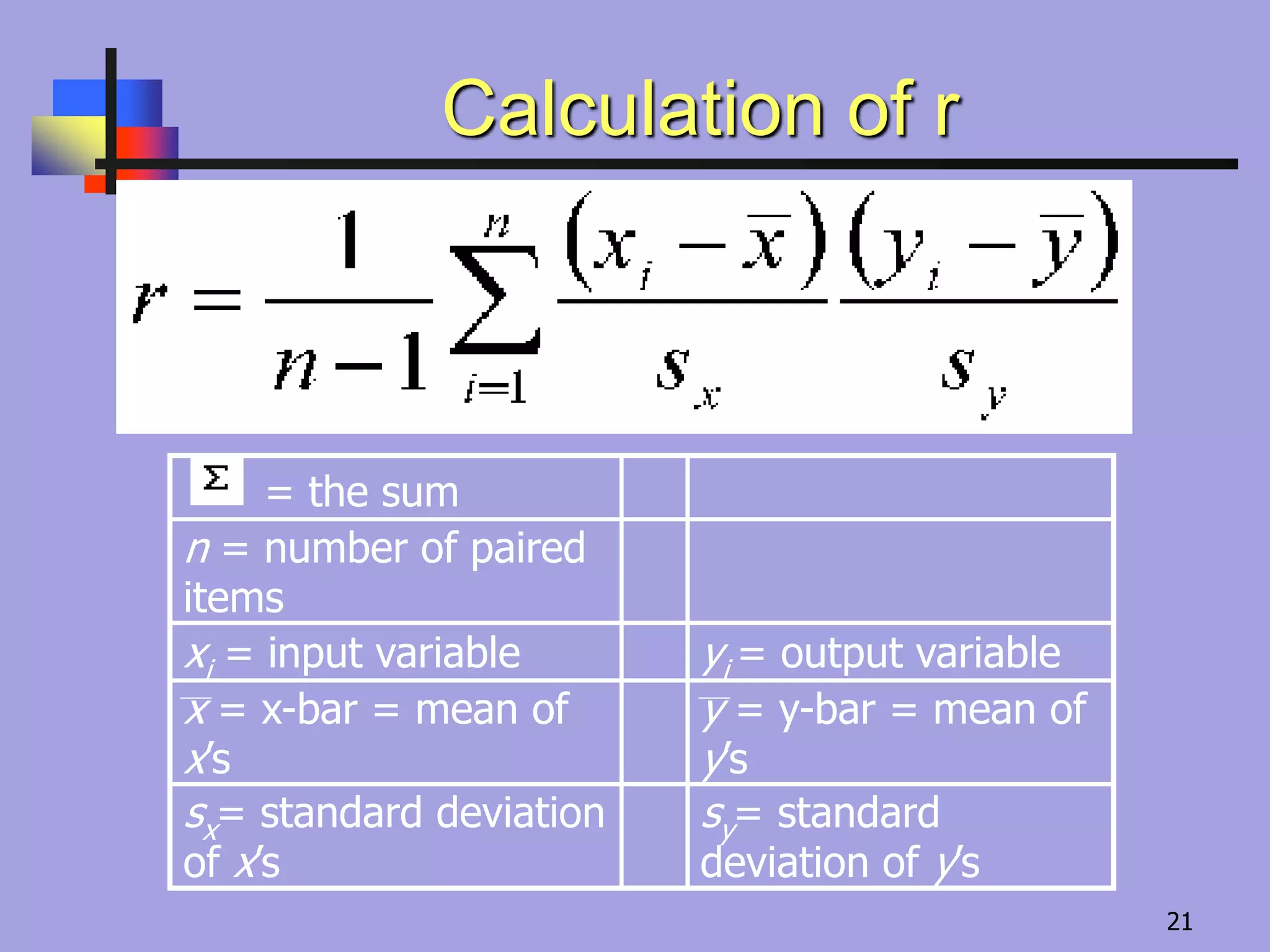
Calculation of r
=the sum
n = number of paired
items
xi = input variable yi = output variable
x = x-bar = mean of
x’s
y = y-bar = mean of
y’s
sx= standard deviation
of x’s
sy= standard
deviation of y’s
21
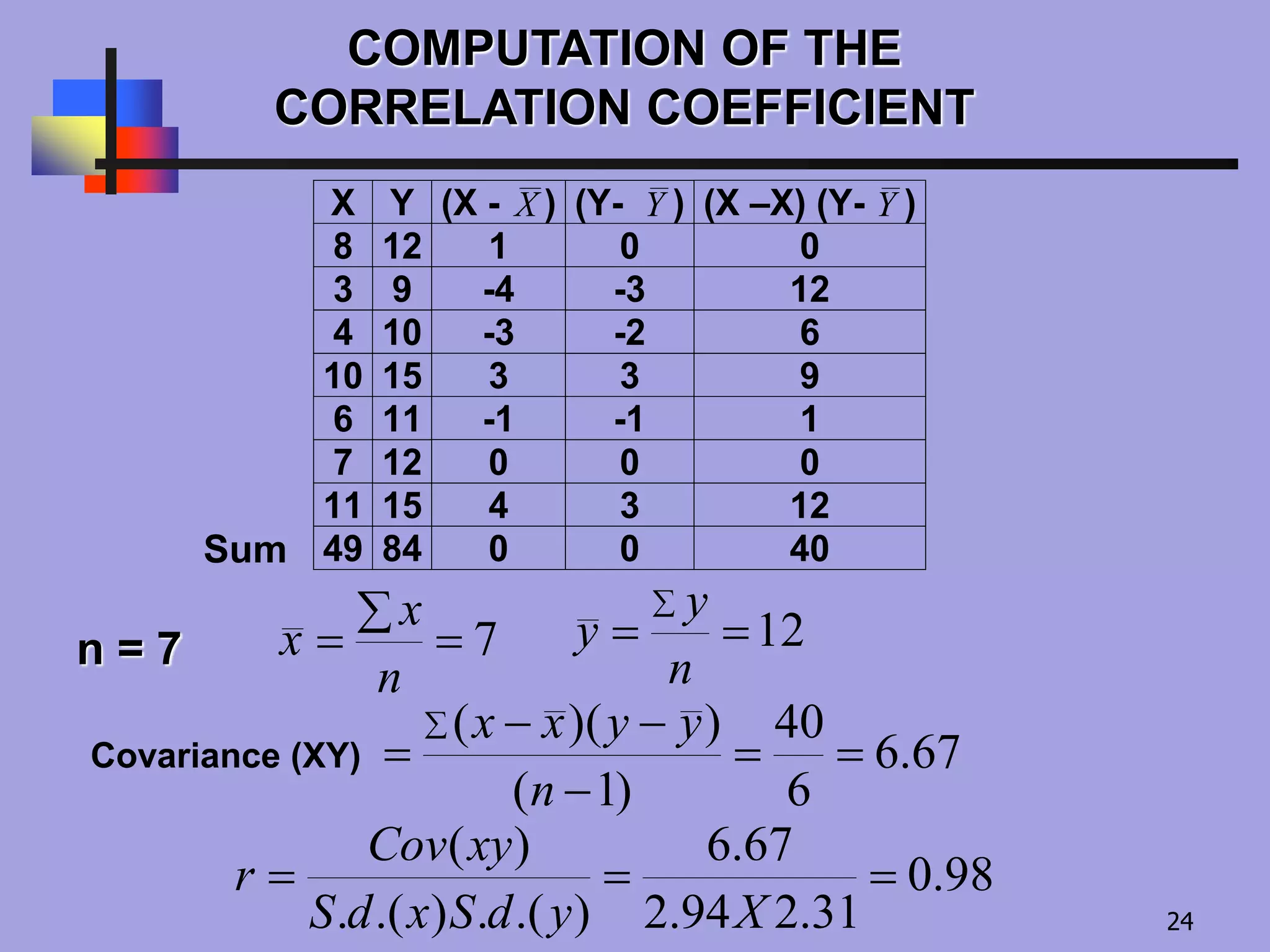
COMPUTATION OF THE
CORRELATIONCOEFFICIENT
Covariance (XY)
X Y (X - X ) (Y- Y ) (X –X) (Y- Y )
8 12 1 0 0
3 9 -4 -3 12
4 10 -3 -2 6
10 15 3 3 9
6 11 -1 -1 1
7 12 0 0 0
11 15 4 3 12
49 84 0 0 40Sum
7
n
x
x 12
n
y
y
67.6
6
40
)1(
))((
n
yyxx
98.0
31.294.2
67.6
).(.).(.
)(
XydSxdS
xyCov
r
n = 7
24
25.
Standard Deviation
Most widelyused measure of
dispersion
σ (Sigma)
Square root of the average of the
squares of deviations
σ = Sqrt [Σ(Xi-Xbar)2/n]
25
26.
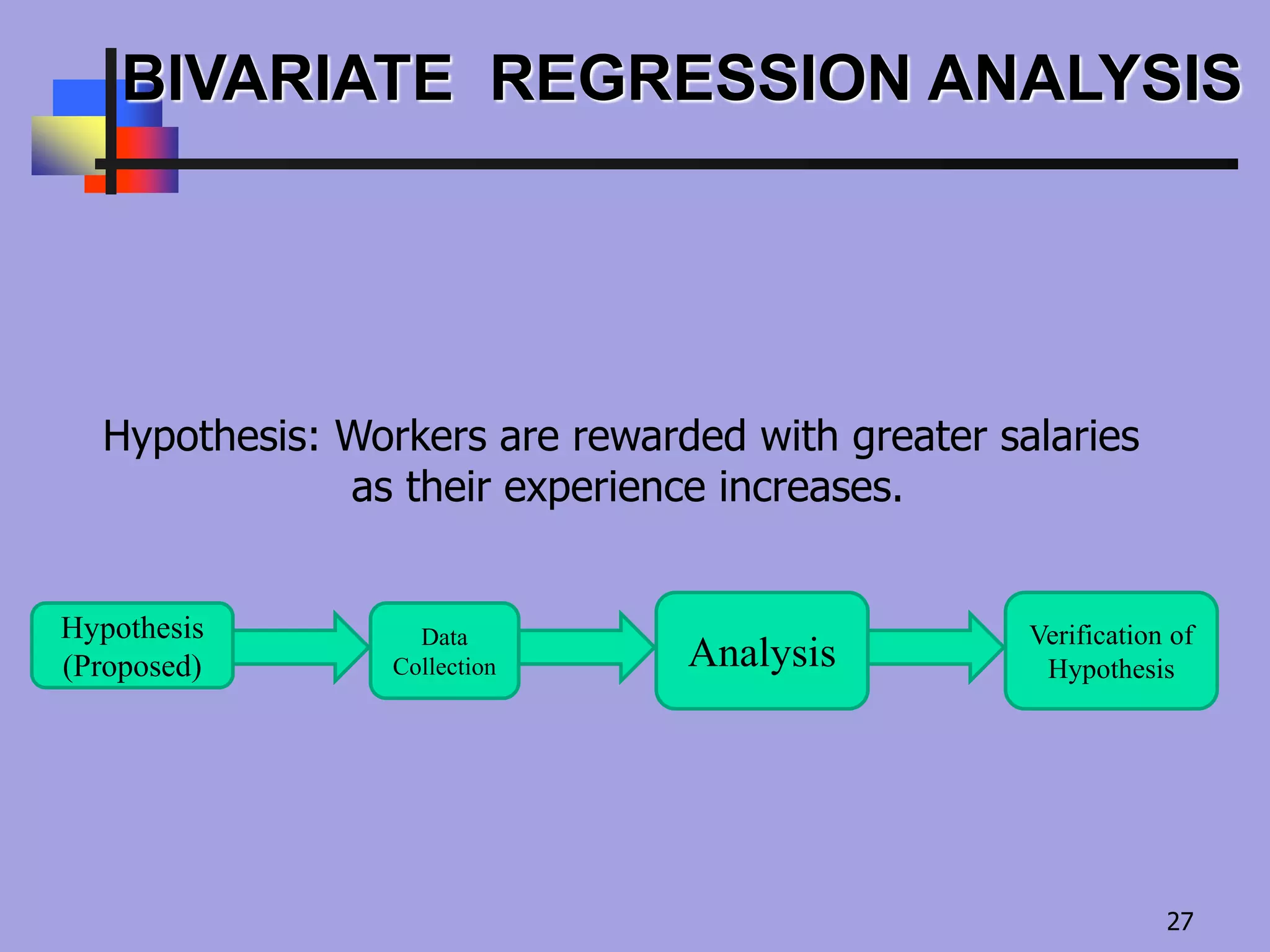
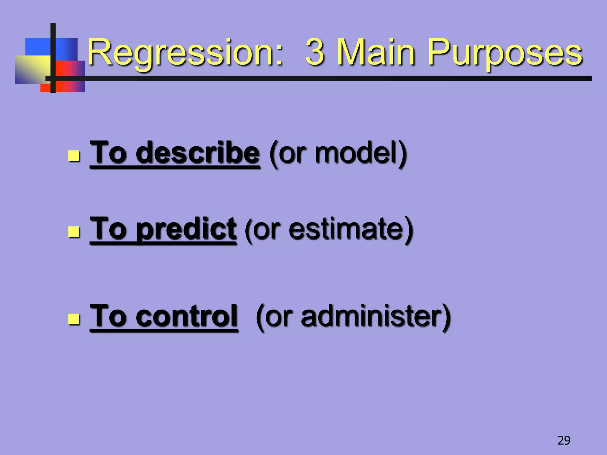
Regression Analysis
BIVARIATE LINEARREGRESSION
Regression : Method of describing the relationship
between two variables
Use : To predict the value of one variable given the other
To use data to analyse relationship.
26
Simple Linear Regression
Statistical method for finding
the “line of best fit”
for one response (dependent)
numerical variable
based on one explanatory
(independent) variable.
28
29.
Regression: 3 MainPurposes
To describe (or model)
To predict (or estimate)
To control (or administer)
29
30.
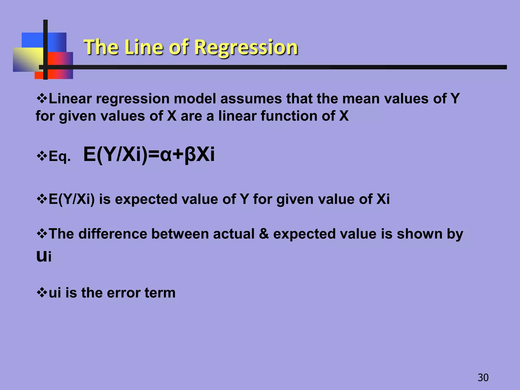
Linear regression modelassumes that the mean values of Y
for given values of X are a linear function of X
Eq. E(Y/Xi)=α+βXi
E(Y/Xi) is expected value of Y for given value of Xi
The difference between actual & expected value is shown by
ui
ui is the error term
The Line of Regression
30
31.
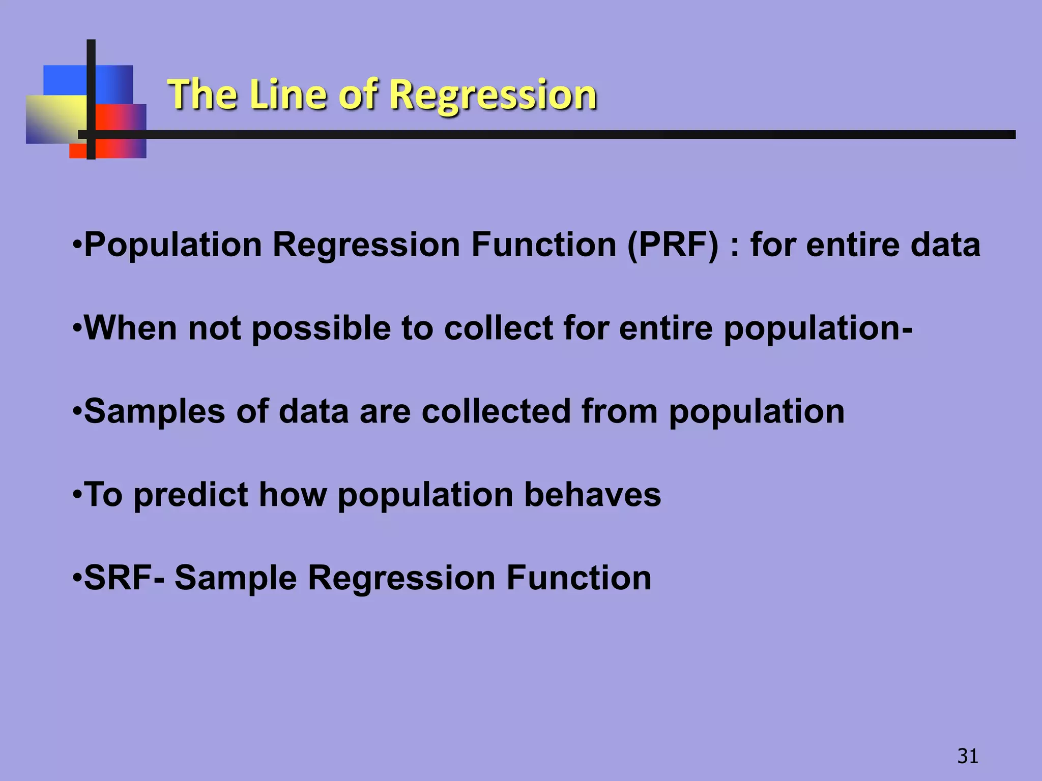
•Population Regression Function(PRF) : for entire data
•When not possible to collect for entire population-
•Samples of data are collected from population
•To predict how population behaves
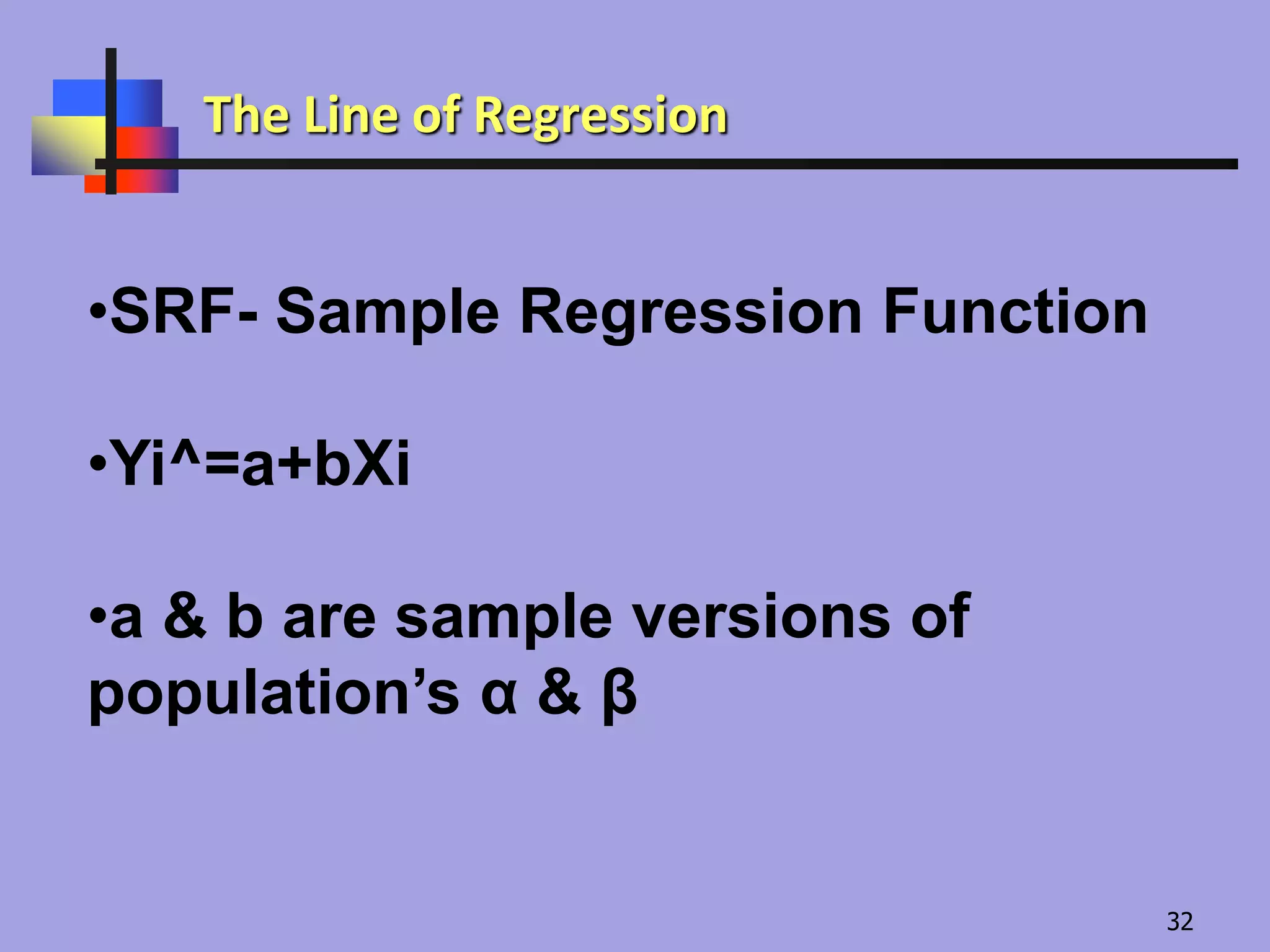
•SRF- Sample Regression Function
The Line of Regression
31
32.
•SRF- Sample RegressionFunction
•Yi^=a+bXi
•a & b are sample versions of
population’s α & β
The Line of Regression
32
33.
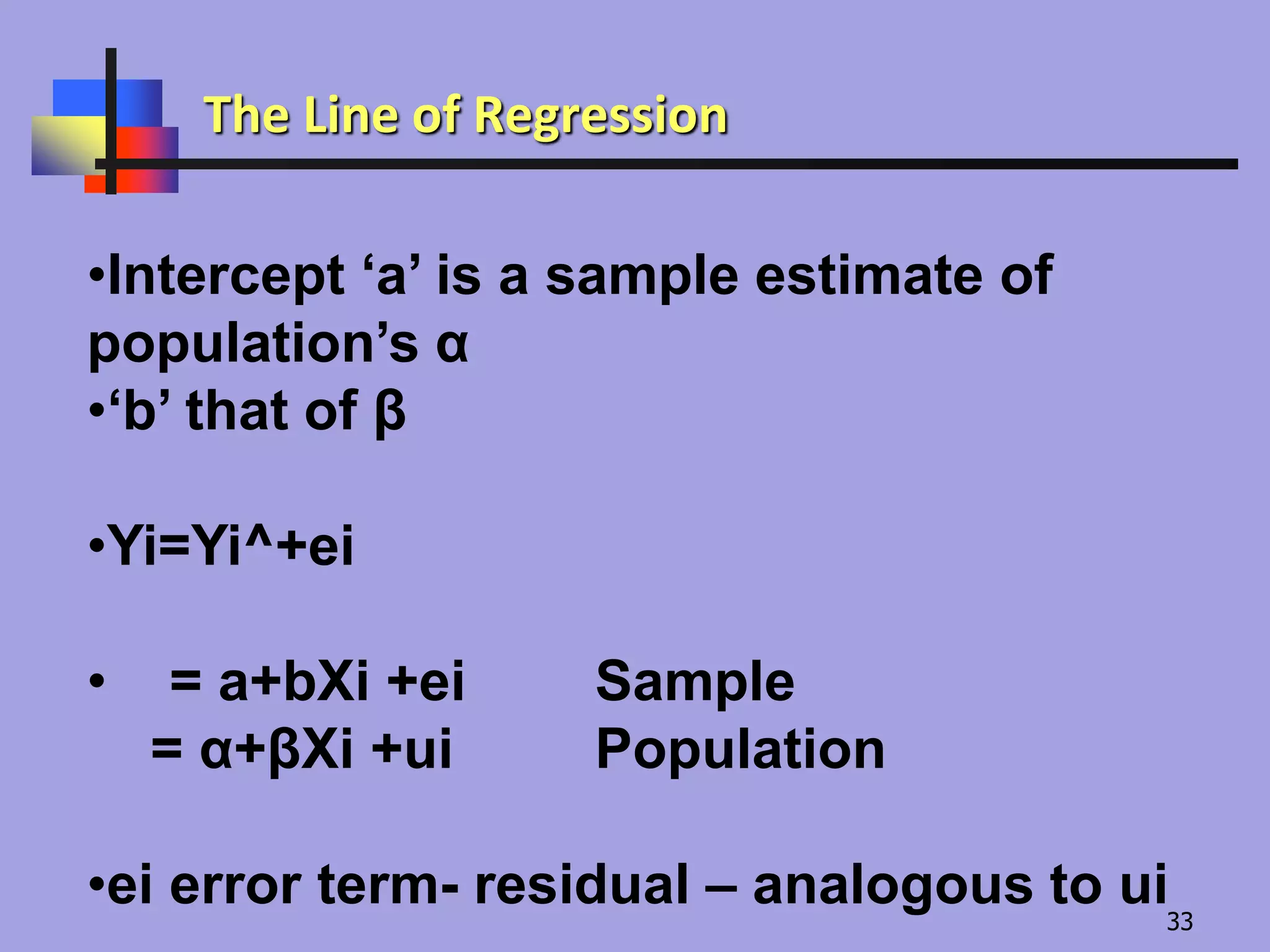
•Intercept ‘a’ isa sample estimate of
population’s α
•‘b’ that of β
•Yi=Yi^+ei
• = a+bXi +ei Sample
= α+βXi +ui Population
•ei error term- residual – analogous to ui
The Line of Regression
33
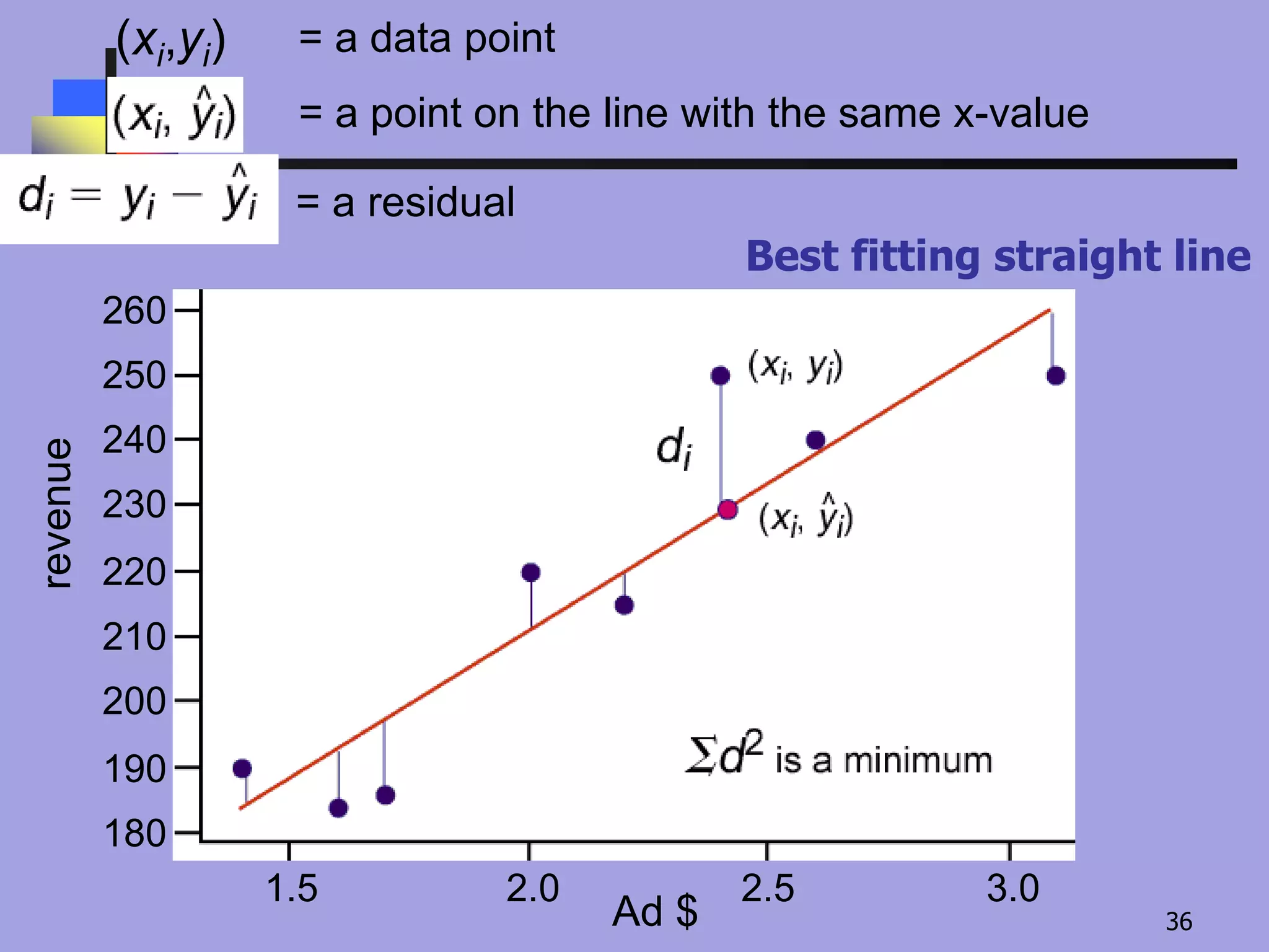
34.
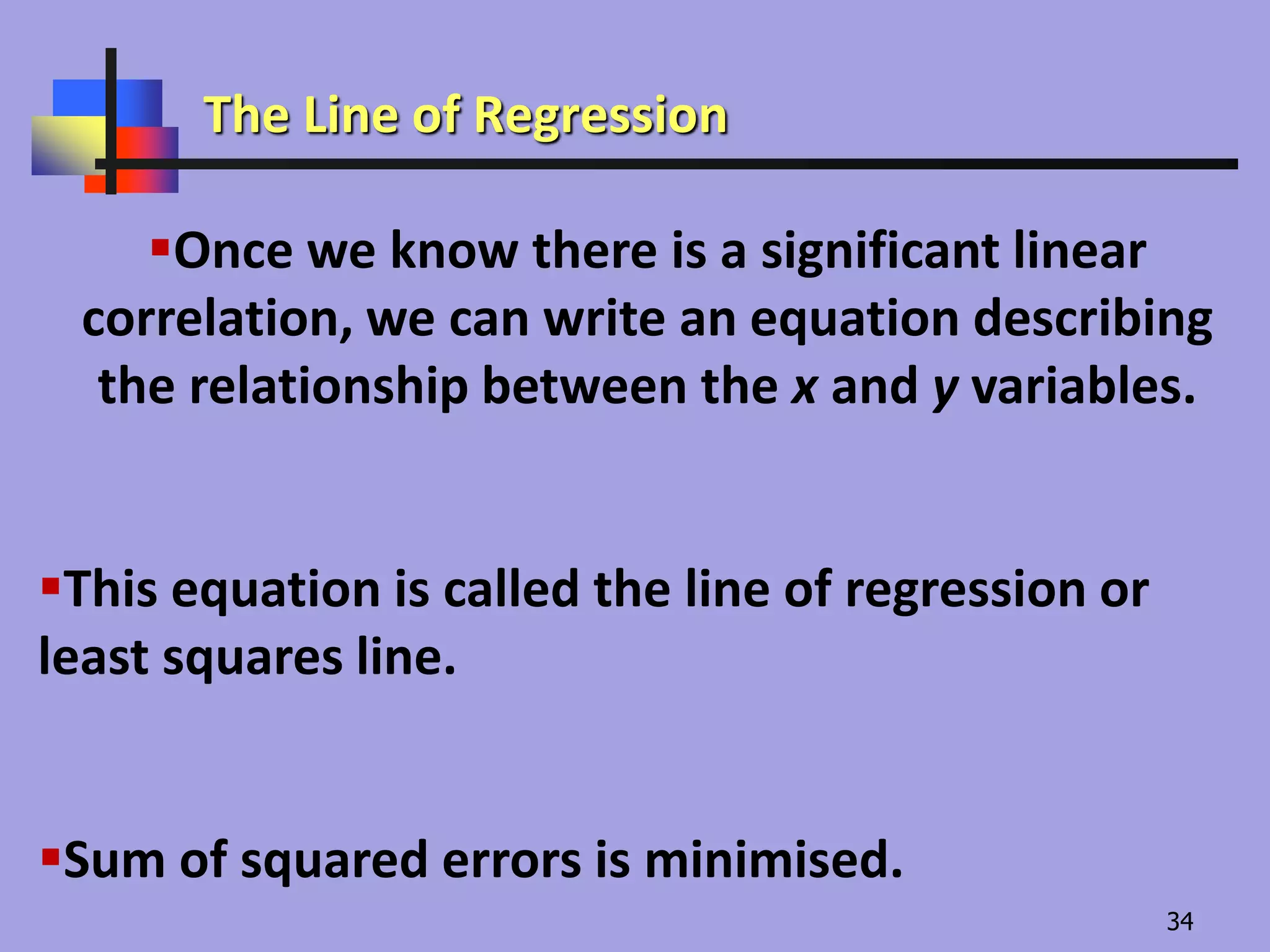
Once we knowthere is a significant linear
correlation, we can write an equation describing
the relationship between the x and y variables.
This equation is called the line of regression or
least squares line.
Sum of squared errors is minimised.
The Line of Regression
34
35.
Least Squares Regression
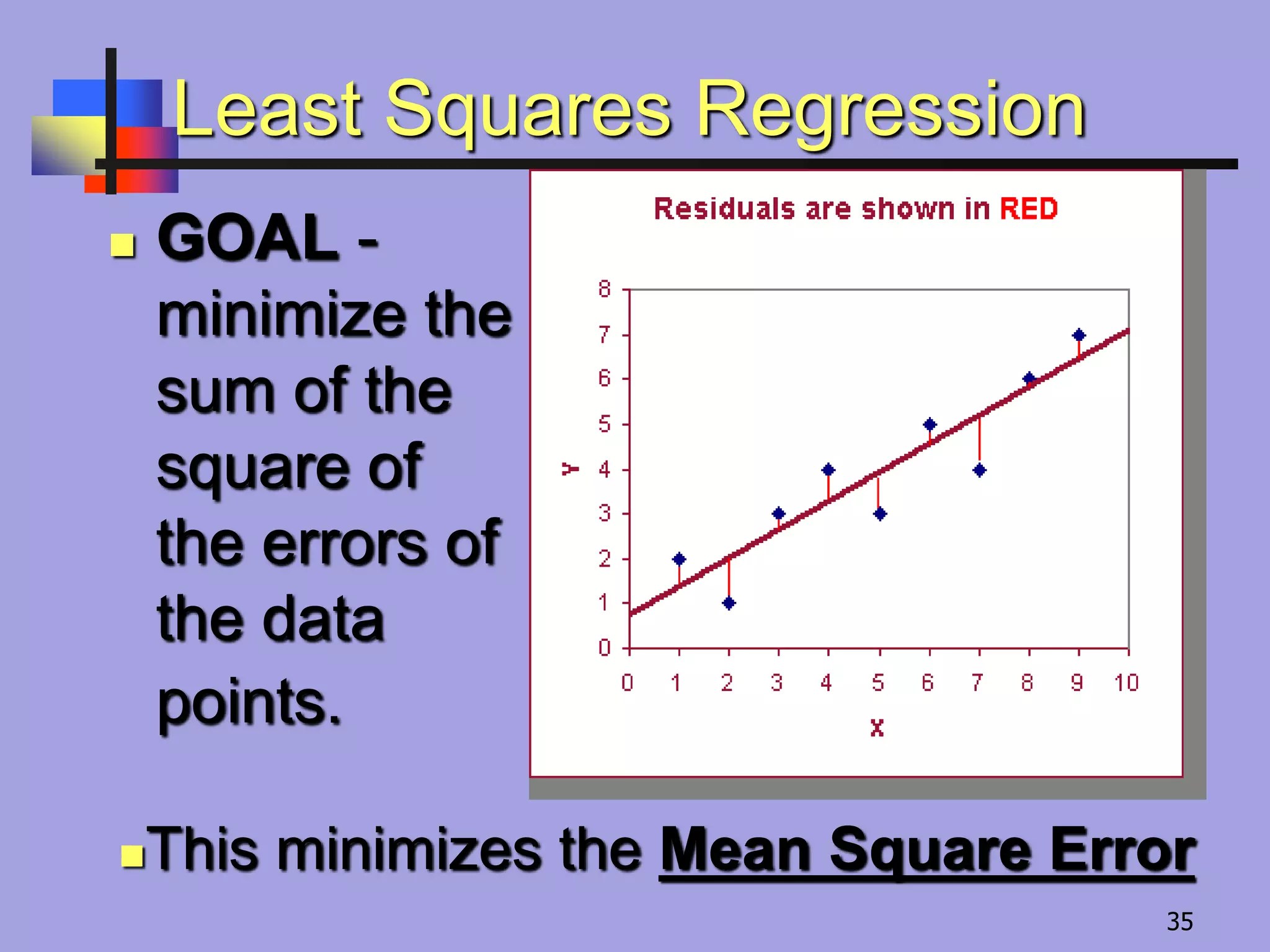
GOAL -
minimize the
sum of the
square of
the errors of
the data
points.
This minimizes the Mean Square Error
35
The equation ofa line may be written as y = a + bXi
where b is the slope of the line and a is the y-
intercept.
The line of regression is:
The slope b is:
The y-intercept a is:
The Line of Regression
37
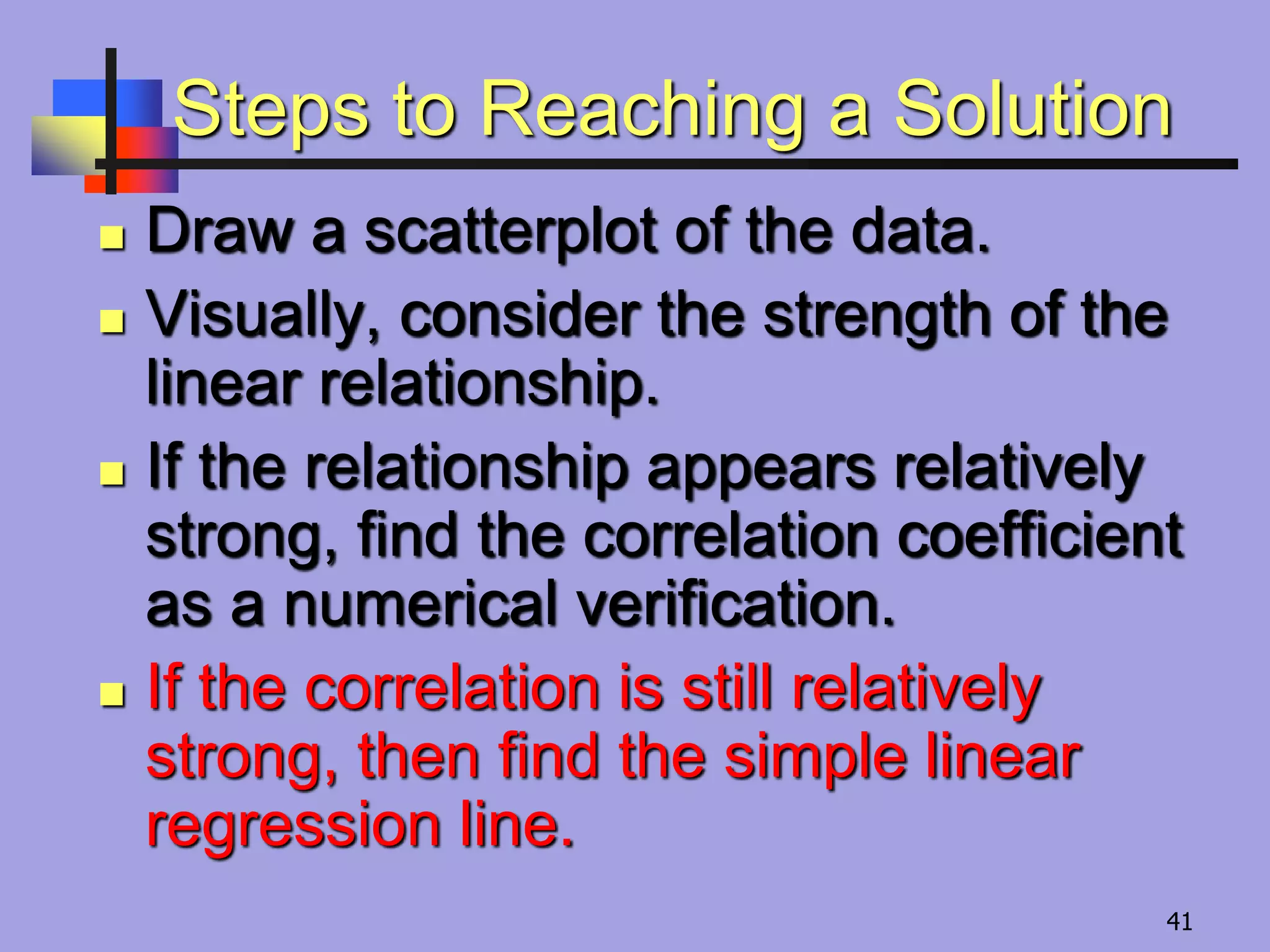
Steps to Reachinga Solution
Draw a scatterplot of the data.
Visually, consider the strength of the
linear relationship.
39
40.
Steps to Reachinga Solution
Draw a scatterplot of the data.
Visually, consider the strength of the
linear relationship.
If the relationship appears relatively
strong, find the correlation coefficient
as a numerical verification.
40
41.
Steps to Reachinga Solution
Draw a scatterplot of the data.
Visually, consider the strength of the
linear relationship.
If the relationship appears relatively
strong, find the correlation coefficient
as a numerical verification.
If the correlation is still relatively
strong, then find the simple linear
regression line.
41
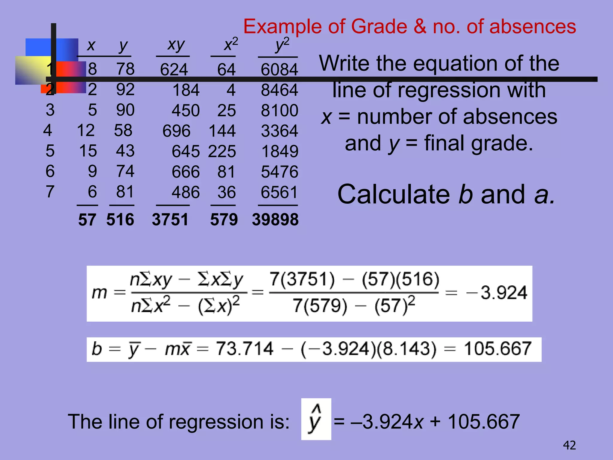
42.
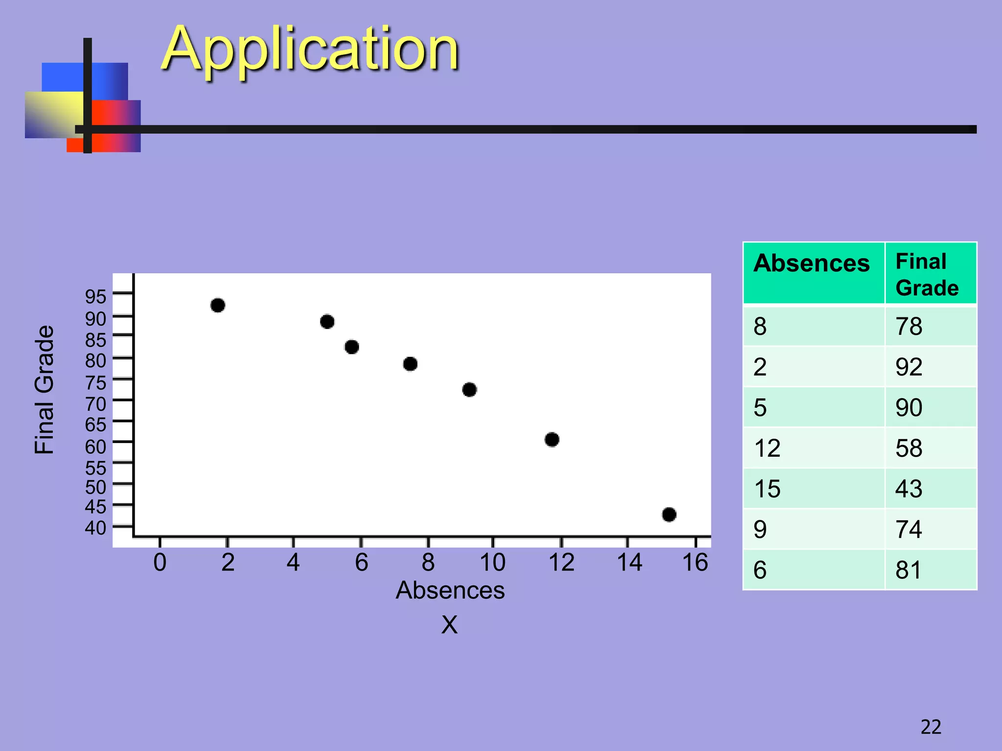
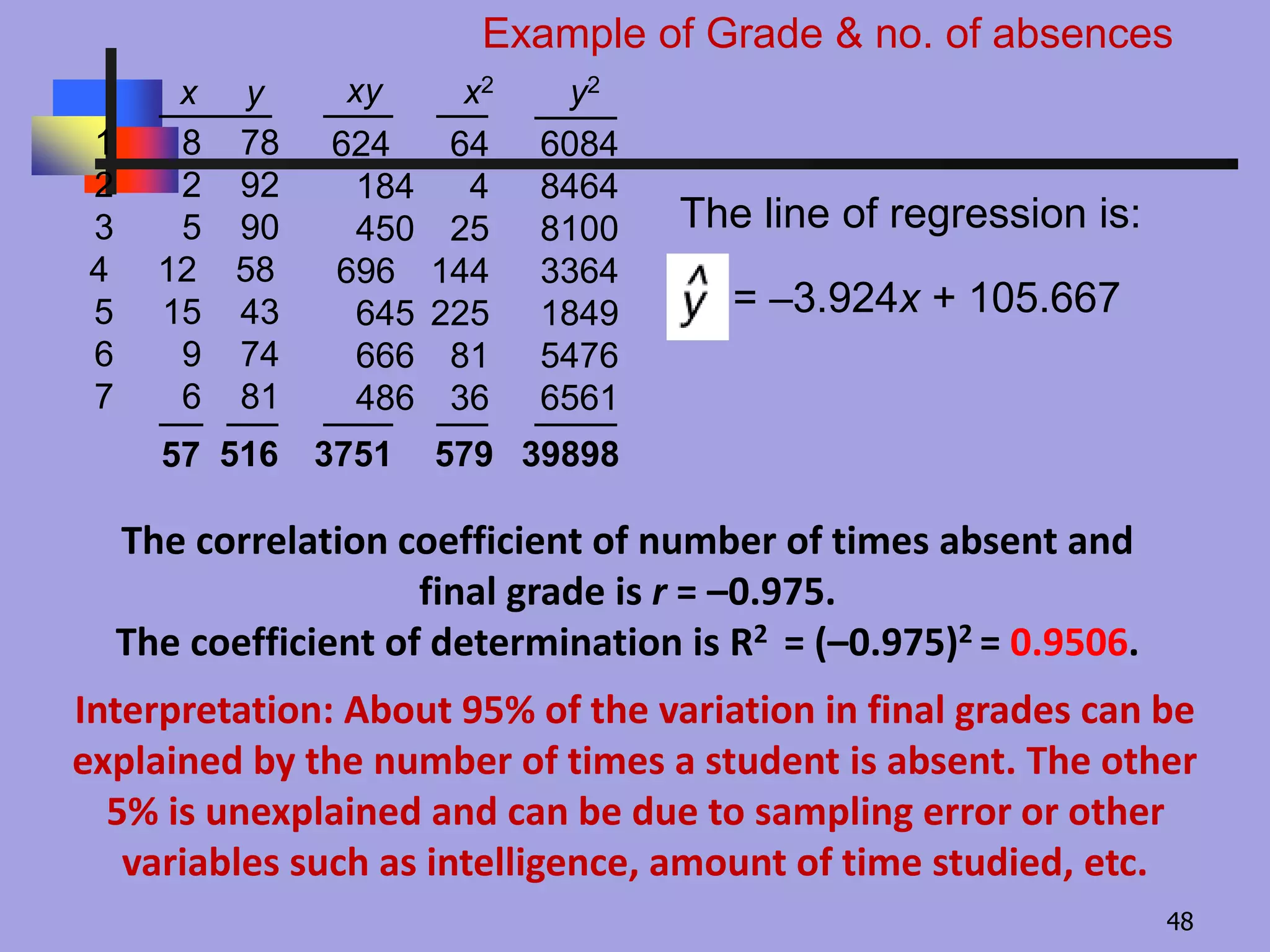
Calculate b anda.
Write the equation of the
line of regression with
x = number of absences
and y = final grade.
The line of regression is: = –3.924x + 105.667
6084
8464
8100
3364
1849
5476
6561
624
184
450
696
645
666
486
57 516 3751 579 39898
1 8 78
2 2 92
3 5 90
4 12 58
5 15 43
6 9 74
7 6 81
64
4
25
144
225
81
36
xy x2 y2x y
Example of Grade & no. of absences
42
43.
0 2 46 8 10 12 14 16
40
45
50
55
60
65
70
75
80
85
90
95
Absences
FinalGrade
m = –3.924 and b = 105.667
The line of regression is:
Note that the point = (8.143, 73.714) is on the line.
The Line of Regression
43
44.
•If CLRM (ClassicalLinear Regression model) assumptions are
satisfied then
•OLS regression line provides the best possible estimate of
population regression line or OLS is
•BLUE- Best Linear Unbiased Estimator
•Linear- Yi= = a+bXi +ei , a & b – raised to power 1
•Unbiased- 1st sample- some value of b
•2nd sample- likely to give different value of b
•Average of all bs=β
•Best- a & b bounce around from sample to sample
•If unbiased- they have mean values equal to α & β
•To be best- they will bounce around
the least.
The Line of Regression
44
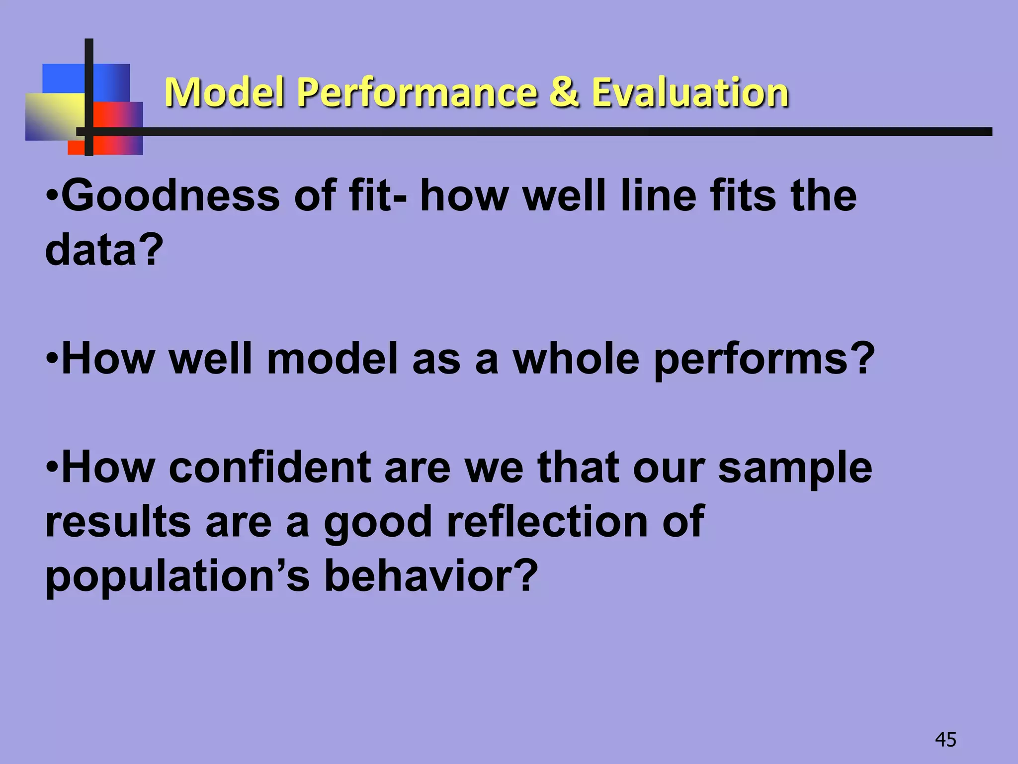
45.
•Goodness of fit-how well line fits the
data?
•How well model as a whole performs?
•How confident are we that our sample
results are a good reflection of
population’s behavior?
Model Performance & Evaluation
45
46.
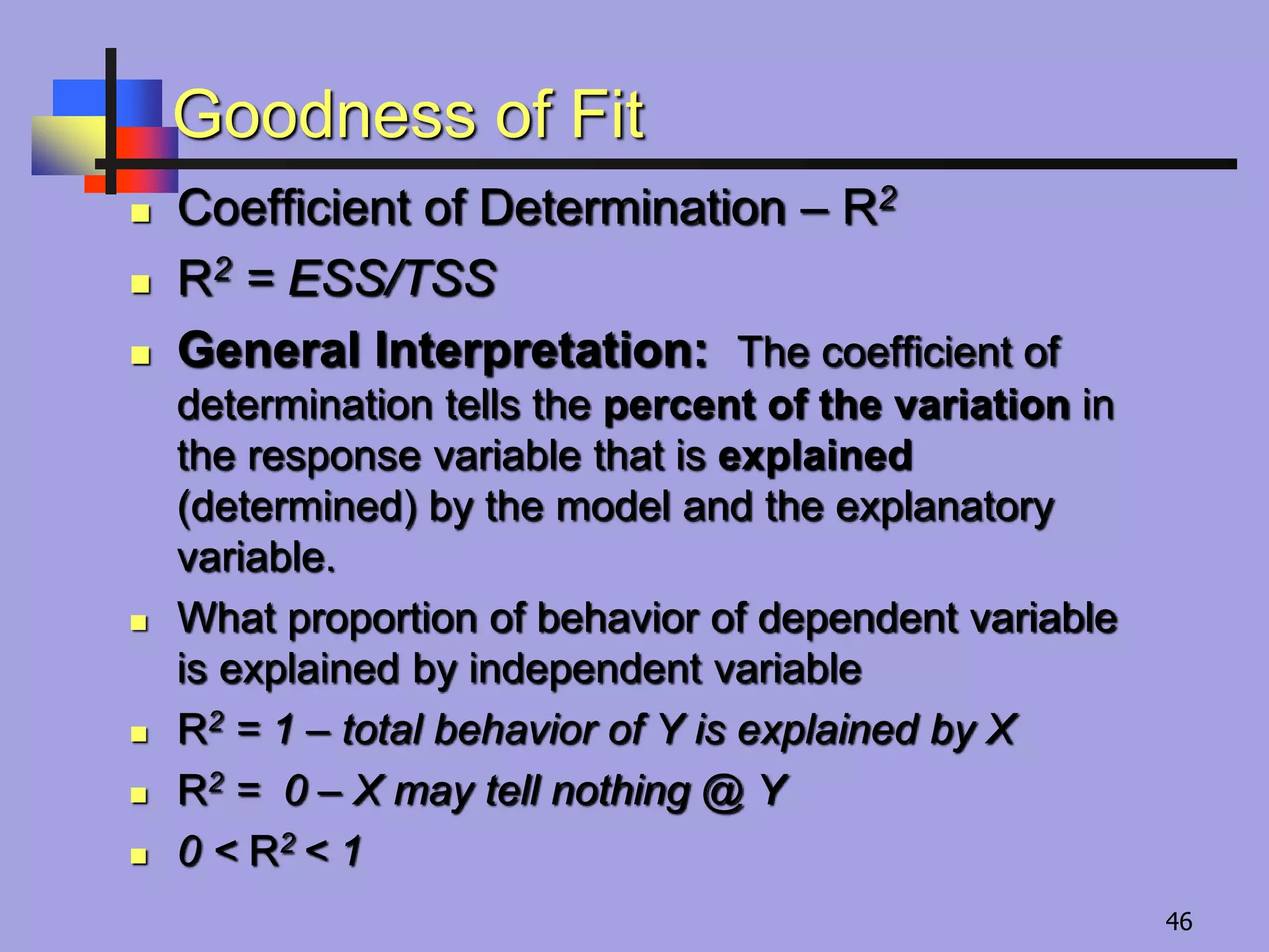
Goodness of Fit
Coefficient of Determination – R2
R2 = ESS/TSS
General Interpretation: The coefficient of
determination tells the percent of the variation in
the response variable that is explained
(determined) by the model and the explanatory
variable.
What proportion of behavior of dependent variable
is explained by independent variable
R2 = 1 – total behavior of Y is explained by X
R2 = 0 – X may tell nothing @ Y
0 ˂ R2 ˂ 1
46
47.
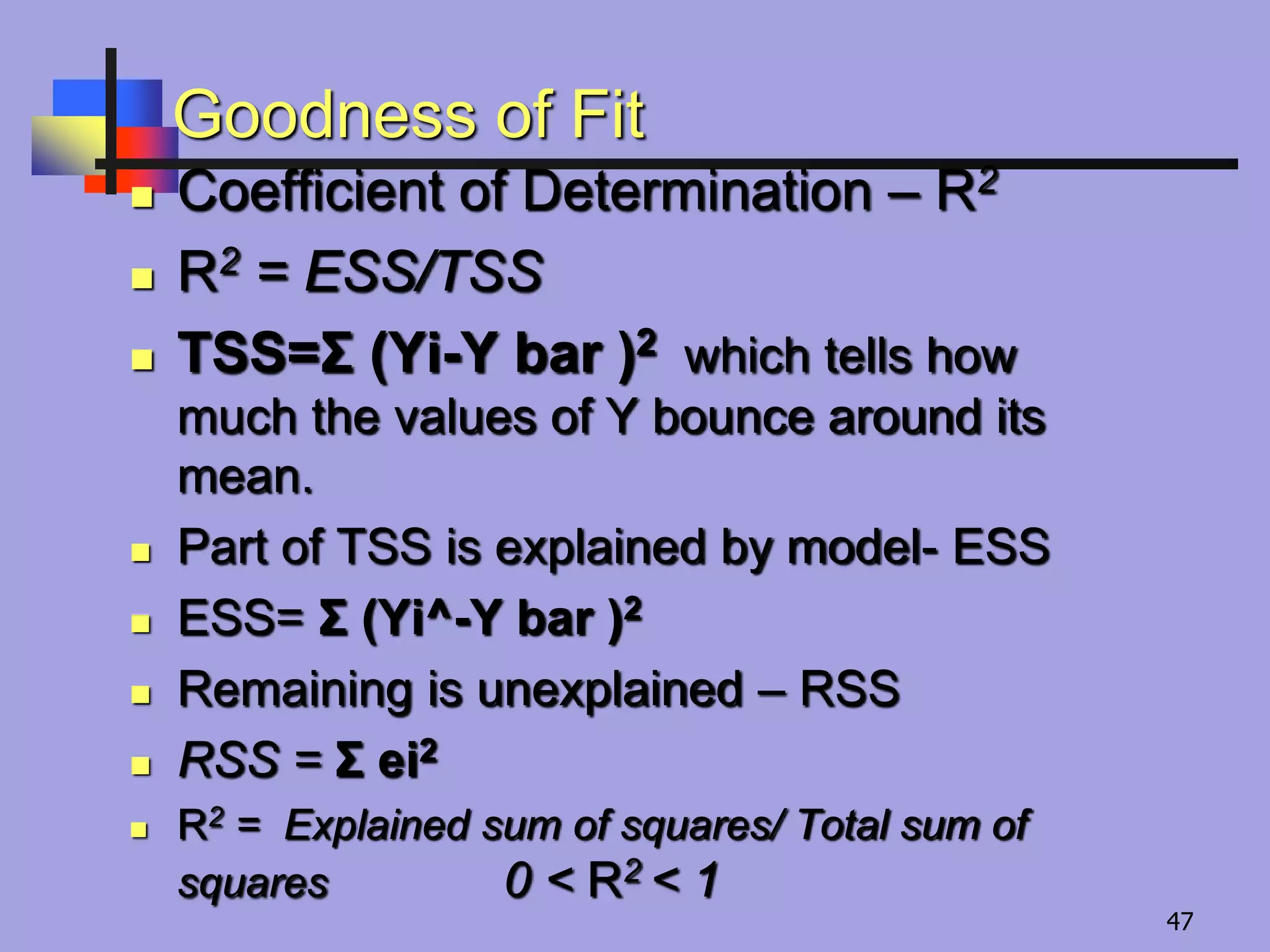
Goodness of Fit
Coefficient of Determination – R2
R2 = ESS/TSS
TSS=Σ (Yi-Y bar )2 which tells how
much the values of Y bounce around its
mean.
Part of TSS is explained by model- ESS
ESS= Σ (Yi^-Y bar )2
Remaining is unexplained – RSS
RSS = Σ ei2
R2 = Explained sum of squares/ Total sum of
squares 0 ˂ R2 ˂ 1
47
48.
The line ofregression is:
= –3.924x + 105.667
6084
8464
8100
3364
1849
5476
6561
624
184
450
696
645
666
486
57 516 3751 579 39898
1 8 78
2 2 92
3 5 90
4 12 58
5 15 43
6 9 74
7 6 81
64
4
25
144
225
81
36
xy x2 y2x y
Example of Grade & no. of absences
The correlation coefficient of number of times absent and
final grade is r = –0.975.
The coefficient of determination is R2 = (–0.975)2 = 0.9506.
Interpretation: About 95% of the variation in final grades can be
explained by the number of times a student is absent. The other
5% is unexplained and can be due to sampling error or other
variables such as intelligence, amount of time studied, etc.
48
5. Interpreting andVisualizing
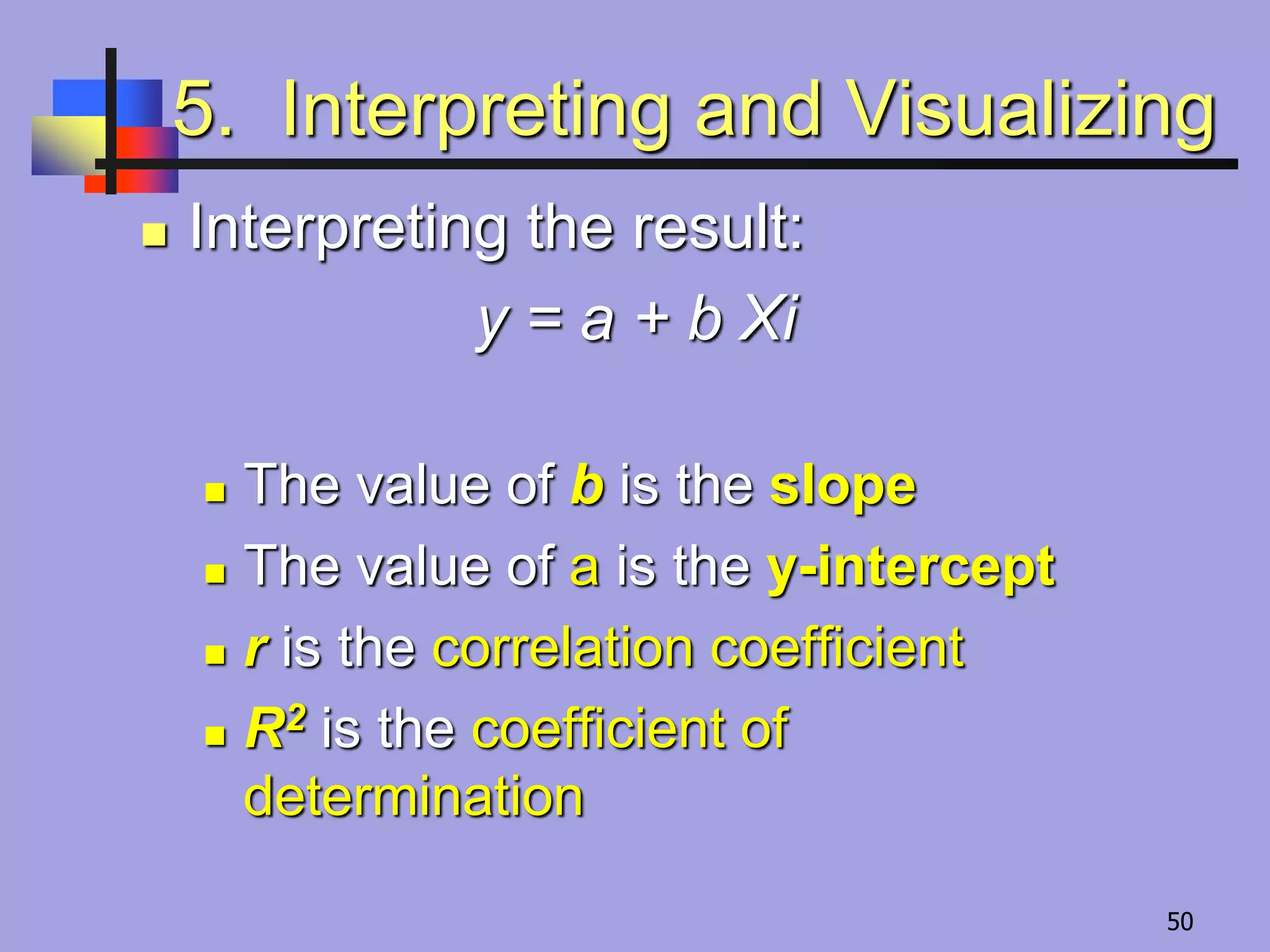
Interpreting the result:
y = a + b Xi
The value of b is the slope
The value of a is the y-intercept
r is the correlation coefficient
R2 is the coefficient of
determination
50
51.
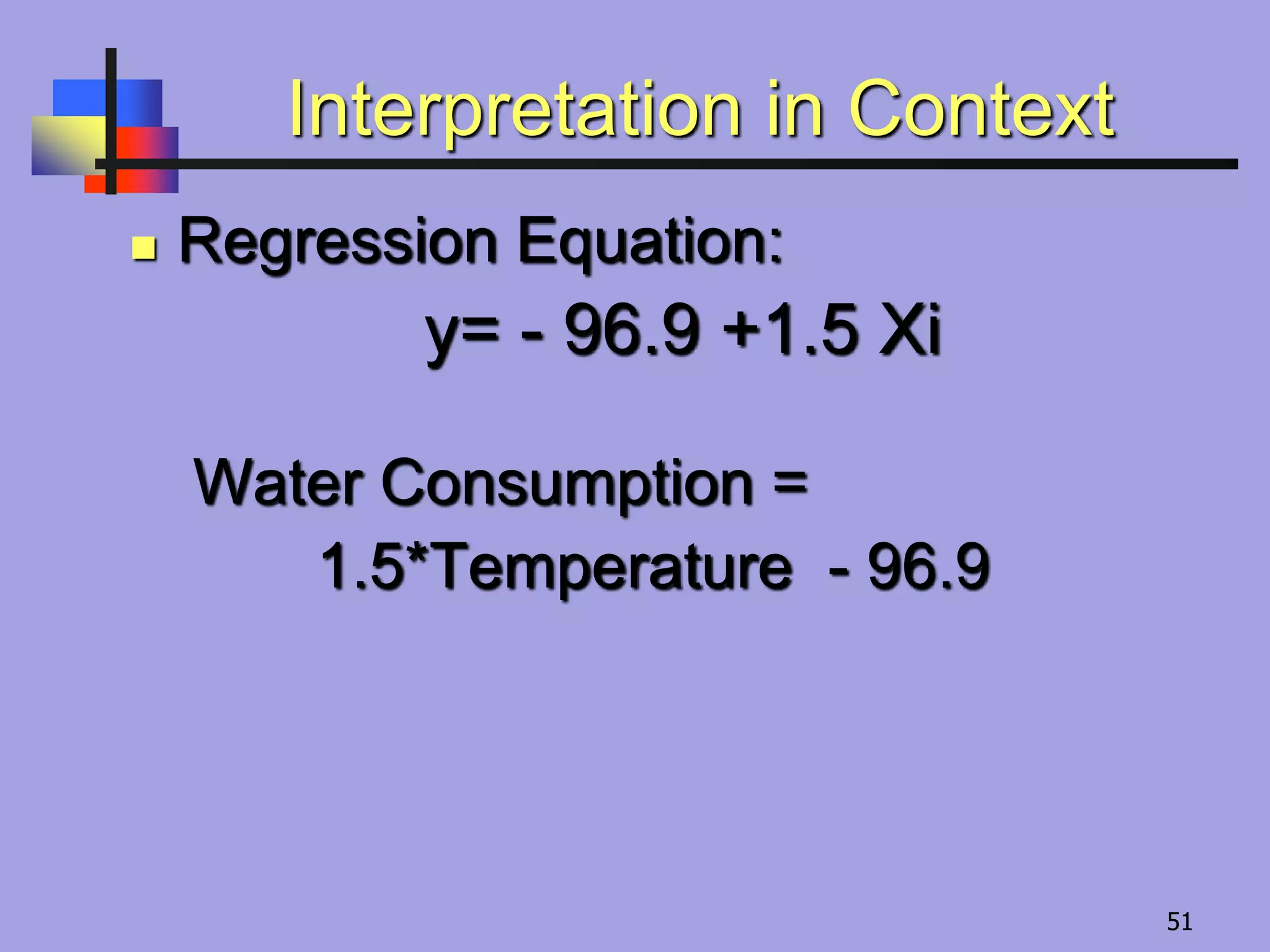
Interpretation in Context
Regression Equation:
y= - 96.9 +1.5 Xi
Water Consumption =
1.5*Temperature - 96.9
51
52.
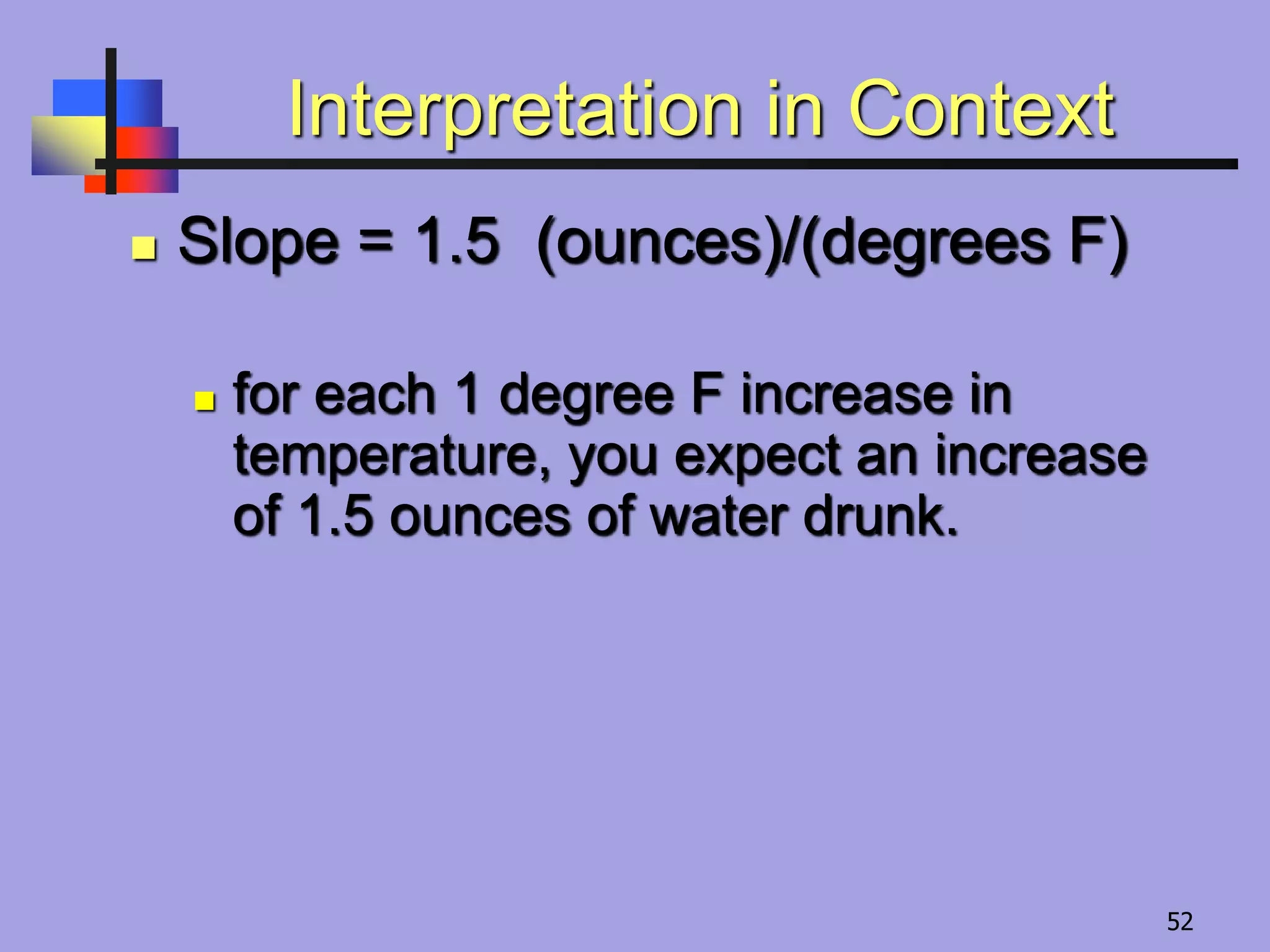
Interpretation in Context
Slope = 1.5 (ounces)/(degrees F)
for each 1 degree F increase in
temperature, you expect an increase
of 1.5 ounces of water drunk.
52
53.
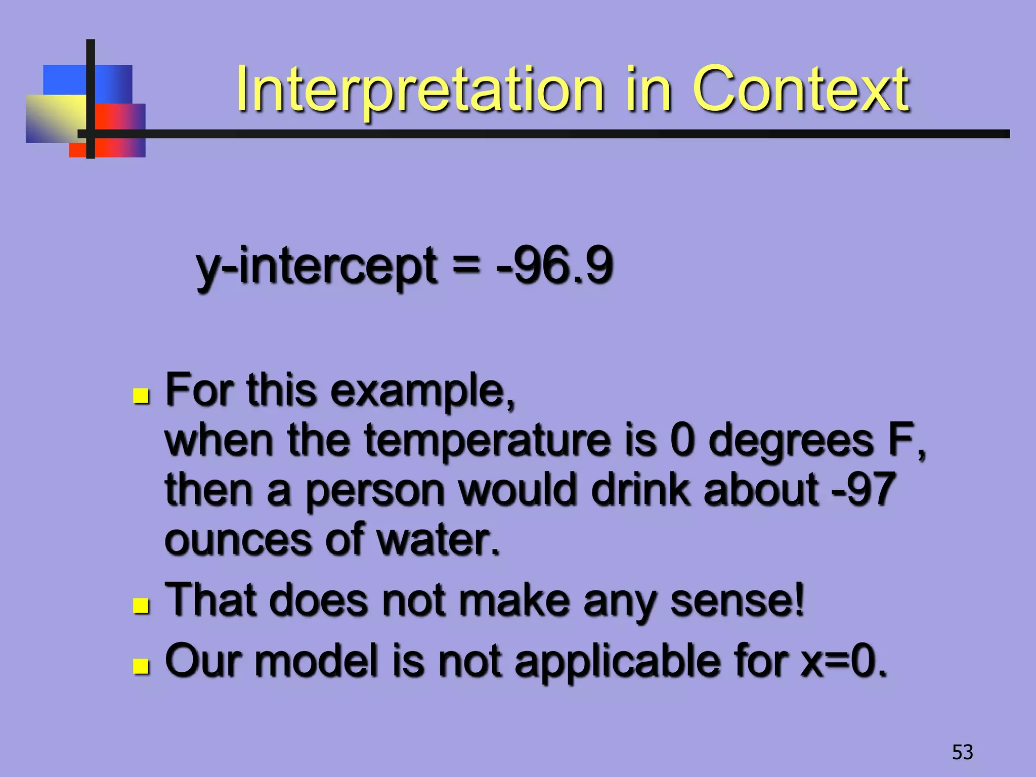
Interpretation in Context
y-intercept= -96.9
For this example,
when the temperature is 0 degrees F,
then a person would drink about -97
ounces of water.
That does not make any sense!
Our model is not applicable for x=0.
53
54.
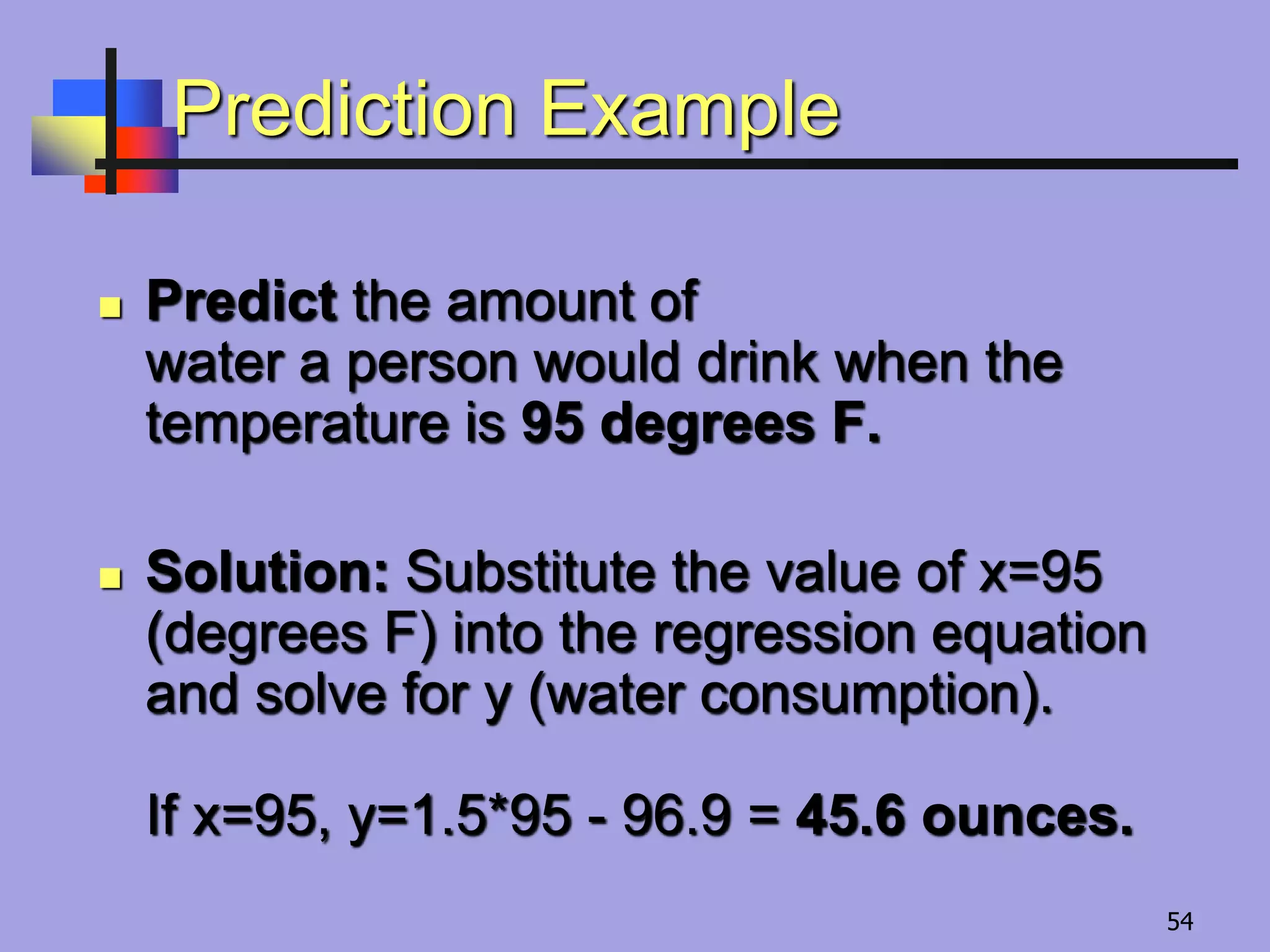
Prediction Example
Predictthe amount of
water a person would drink when the
temperature is 95 degrees F.
Solution: Substitute the value of x=95
(degrees F) into the regression equation
and solve for y (water consumption).
If x=95, y=1.5*95 - 96.9 = 45.6 ounces.
54
55.
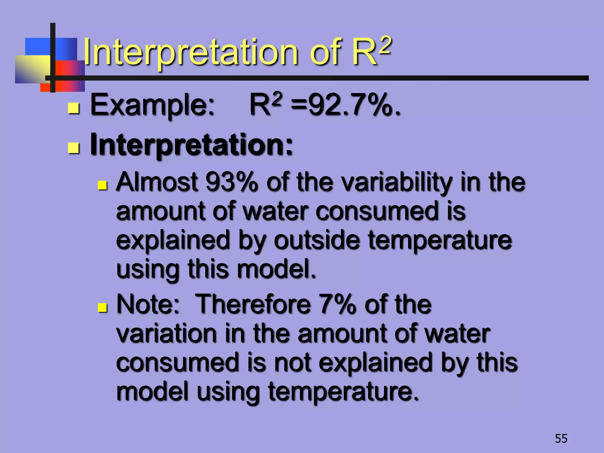
Interpretation of R2
Example: R2 =92.7%.
Interpretation:
Almost 93% of the variability in the
amount of water consumed is
explained by outside temperature
using this model.
Note: Therefore 7% of the
variation in the amount of water
consumed is not explained by this
model using temperature.
55
56.
Standard Error
Positivesquare root of the variance of
error
It is a measure used to judge the reliability
of a & b as estimates of α & β
Two imp things @ std. error
Its unit is same as dependent variable
Its size relative to the value of estimated
coefficient
t stat ( t statistic) gives the size of std. error
relative to the estimated coefficient
t stat = estimated coefficient / std. error
Positive values of t stat above 5 – corresponding
coeff. Is a reliable estimate of α or β 56
57.
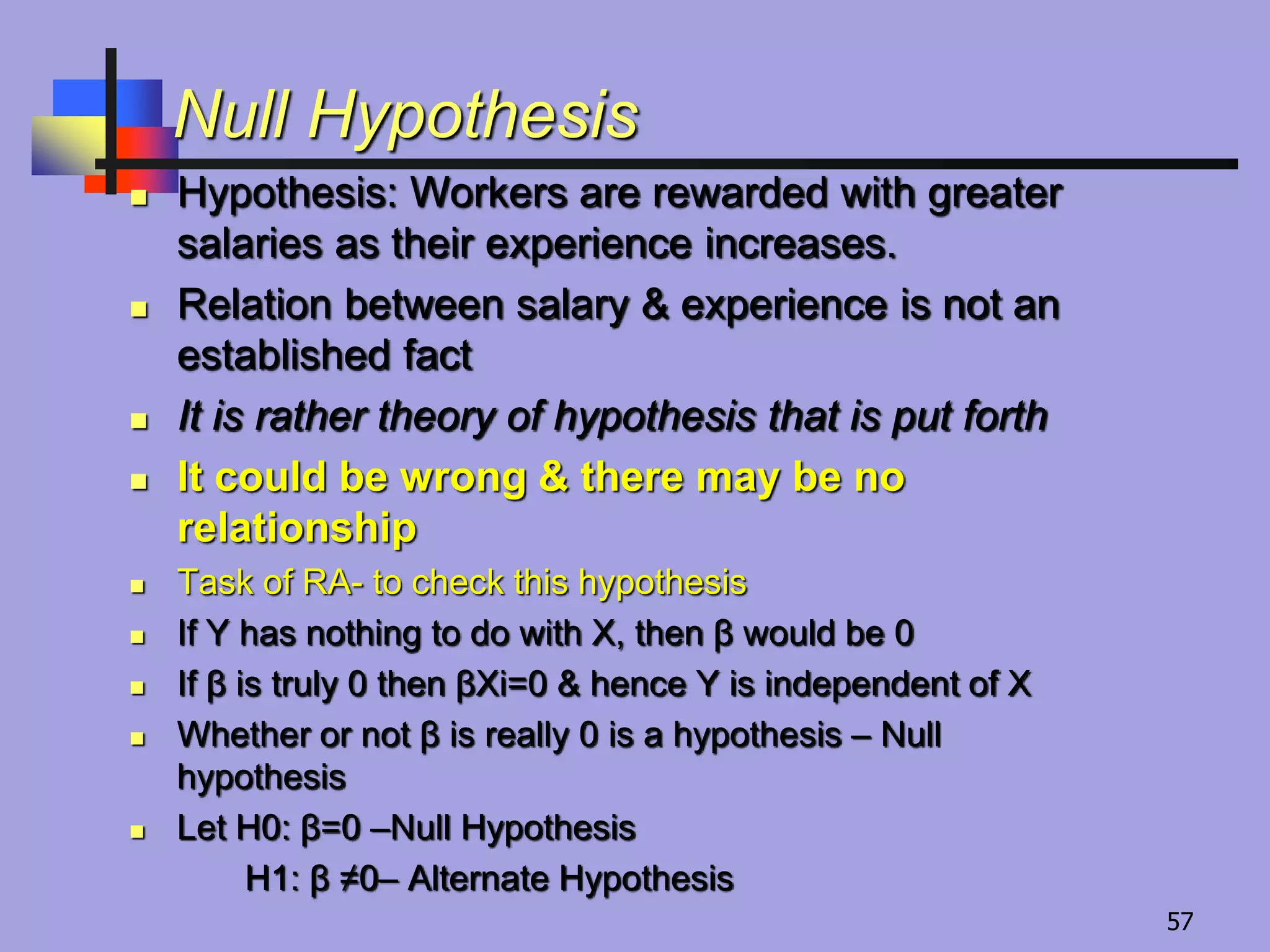
Null Hypothesis
Hypothesis:Workers are rewarded with greater
salaries as their experience increases.
Relation between salary & experience is not an
established fact
It is rather theory of hypothesis that is put forth
It could be wrong & there may be no
relationship
Task of RA- to check this hypothesis
If Y has nothing to do with X, then β would be 0
If β is truly 0 then βXi=0 & hence Y is independent of X
Whether or not β is really 0 is a hypothesis – Null
hypothesis
Let H0: β=0 –Null Hypothesis
H1: β ≠0– Alternate Hypothesis
57
58.
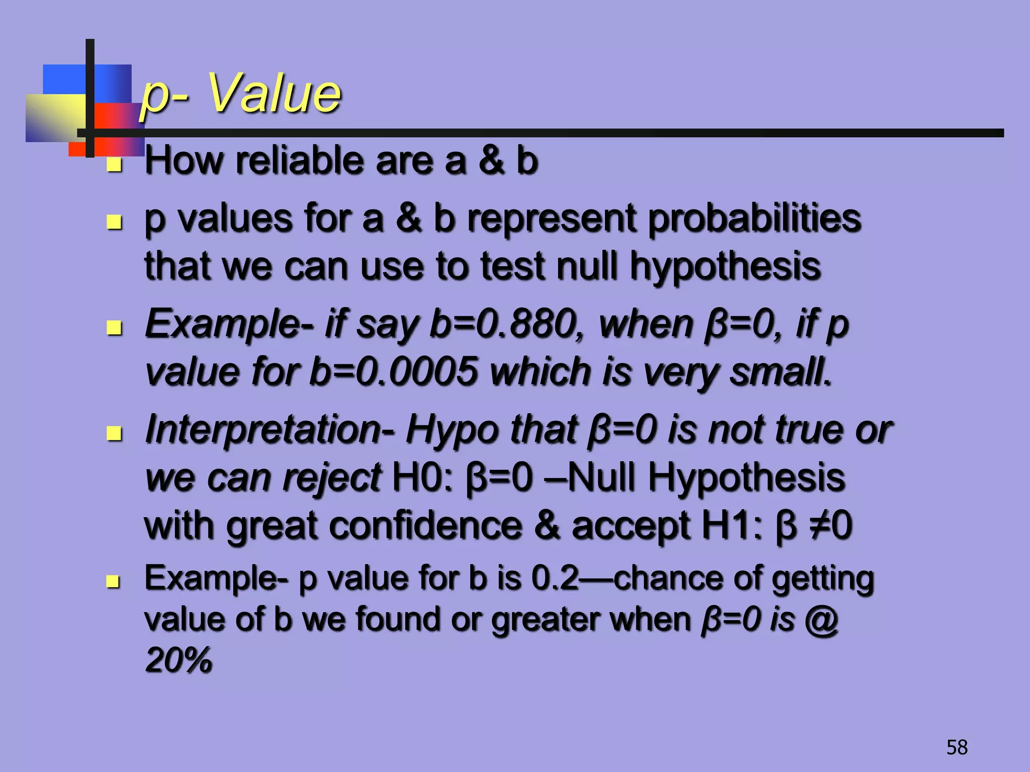
p- Value
Howreliable are a & b
p values for a & b represent probabilities
that we can use to test null hypothesis
Example- if say b=0.880, when β=0, if p
value for b=0.0005 which is very small.
Interpretation- Hypo that β=0 is not true or
we can reject H0: β=0 –Null Hypothesis
with great confidence & accept H1: β ≠0
Example- p value for b is 0.2—chance of getting
value of b we found or greater when β=0 is @
20%
58
59.
When to rejectNull Hypothesis
When associated p values are
0.05 or smaller
95% confidence level
In some cases- p values of 0.1 or
smaller are used
90% confidence level
59
![6084
8464
8100
3364
1849
5476
6561
624
184
450
696
645
666
486
57 516 3751 579 39898
1 8 78
2 2 92
3 5 90
4 12 58
5 15 43
6 9 74
7 6 81
64
4
25
144
225
81
36
xy x2 y2
Computation of r
x y
Σ
r=Cov(xy) / [Sd(x) x Sd(y)]
23](https://image.slidesharecdn.com/correlationregressionppt-170510083621/75/Correlation-and-Regression-ppt-23-2048.jpg)
![Standard Deviation
Most widely used measure of
dispersion
σ (Sigma)
Square root of the average of the
squares of deviations
σ = Sqrt [Σ(Xi-Xbar)2/n]
25](https://image.slidesharecdn.com/correlationregressionppt-170510083621/75/Correlation-and-Regression-ppt-25-2048.jpg)


![[DSC Europe 25] Dragana Ilic - AI for Big Data in Astronomy.pptx](https://cdn.slidesharecdn.com/ss_thumbnails/8palya86qaatvjhva1ms-2-dragana-ilic-ai-ilic-251208151906-652b819c-thumbnail.jpg?width=640&height=640&fit=bounds)


![[DSC Europe 25] Vid Stimac - Policy Parsimony: Between Oversimplifying and Ov...](https://cdn.slidesharecdn.com/ss_thumbnails/eqlepagzqp2rhg3gbluh-dsc-stimac-251120-251205090438-059e7f54-thumbnail.jpg?width=640&height=640&fit=bounds)


![[DSC Europe 25] Dusan Jovicic - AI Story: From on-prem to cloud and back agai...](https://cdn.slidesharecdn.com/ss_thumbnails/8kp49m6uq22ifnbwhfnk-2-251205085715-964d11a6-thumbnail.jpg?width=640&height=640&fit=bounds)