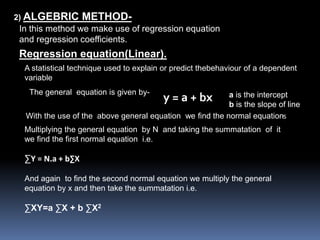
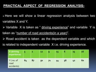
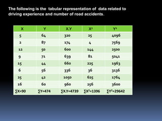
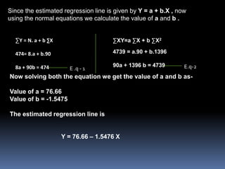
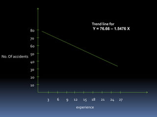
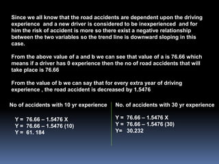
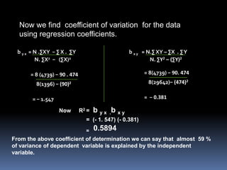
BUSINESS STATISTICS 
PRESENTATION 
ON 
REGRESSION ANALYSIS 
PRESENTED BY-HARI 
BHATTARAI 
MBA 1STYEAR
OBJECTIVES OF THE PRESENTATION- 
What is regression analysis 
Types and methods of regression analysis 
Practical aspect of regression analysis with an 
example
INTRODUCTION- 
Regression analysis is the statistical tool which is 
employed for the purpose of forecasting or making 
estimates 
 Here we make use of various mathematical formulas 
and assumptions to describe a real world situation. 
 In every situation, estimation becomes easy once it is 
known that the variable to be estimated is related to and 
dependent to some other variable.
For making estimates we first have to model the relationship 
between the variable involved . 
Models can me broadly be classified into – 
Linear regression- 
 Linear regression analysis is a powerful technique used for 
predicting the unknown value of a variable from the known 
value of another variable. 
More precisely, if X and Y are two related variables, then 
linear regression analysis helps us to predict the value of Y 
for a given value of X or vice verse. 
For example age of a human being and maturity are related 
variables. Then linear regression analyses can predict level 
of maturity given age of a human being.
Multiple regression- 
 Multiple regression analysis is a powerful technique 
used for predicting the unknown value of a variable from 
the known value of two or more variables- also called the 
predictors. 
Multiple regression analysis helps us to predict the value 
of Y for given values of X1, X2, …, Xk. 
For example the yield of rice per acre depends upon 
quality of seed, fertility of soil, fertilizer used, temperature, 
rainfall. If one is interested to study the joint affect of all 
these variables on rice yield, one can use this technique.
Dependent and Independent Variables- 
 By linear regression, we mean models with just one 
independent and one dependent variable. The variable whose 
value is to be predicted is known as the dependent variable 
and the one whose known value is used for prediction is 
known as the independent variable. 
 By multiple regression, we mean models with just one 
dependent and two or more independent variables. The 
variable whose value is to be predicted is known as the 
dependent variable and the ones whose known values are 
used for prediction are known independent variables.
Methods of solving regression models- 
1) GRAPHICAL METHOD-In 
this graphical method the average relationship 
between the dependent variable and independent 
variable is expressed by a line called “line of best fit”. 
Example: Experience( in years) Income( in ‘000) 
15 150 
10 120 
5 60 
3 40 
8 70 
9 90
2 4 6 8 10 12 14 16 
210 
180 
150 
120 
90 
60 
30 
18 
240 
0 
Line of best fit 
income 
experience
2) ALGEBRIC METHOD-In 
this method we make use of regression equation 
and regression coefficients. 
Regression equation(Linear). 
A statistical technique used to explain or predict thebehaviour of a dependent 
variable 
The general equation is given by- y = a + bx a is the intercept 
b is the slope of line 
With the use of the above general equation we find the normal equations 
Multiplying the general equation by N and taking the summatation of it 
we find the first normal equation i.e. 
ΣY = N.a + bΣX 
And again to find the second normal equation we multiply the general 
equation by x and then take the summatation i.e. 
ΣXY=a ΣX + b ΣX2
Regression equation(Multiple). 
General equation => y = a + b1 x1 + b2x2 + .........+ bnxn 
Normal equations for multiple regression are: 
ΣY = N.a + b1ΣX1 + b2ΣX2 
ΣX1Y= a ΣX1 + b1 Σ X1 
2 + b2Σ X1 . X2 
2 
ΣX2Y= a ΣX2 + b1 Σ X1 . X2 + b2Σ X2
Lines of Regression 
There are two lines of regression- that of Y on X and X on Y. 
The line of regression of Y on X is given by Y = a + bX where a and b 
are unknown constants known as intercept and slope of the equation. 
This is used to predict the unknown value of variable Y when value of 
variable X is known. 
On the other hand, the line of regression of X on Y is given by X = c + dY 
which is used to predict the unknown value of variable X using the 
known value of variable Y. 
Often, only one of these lines make sense. 
Exactly which of these will be appropriate for the analysis in hand will 
depend on labeling of dependent and independent variable in the 
problem to be analyzed.
Regression coefficients- 
The coefficient of X in the line of regression of Y on X is called the 
regression coefficient of Y on X and is denoted by b y x 
It represents change in the value of dependent variable (Y)corresponding to 
unit change in the value of independent variable (X). 
And similarly the coefficient of Y in the line of regression of X on Y is 
called coefficient of X on Y and is denoted by b x y . 
The two regression co-efficient are byx and bxy . 
The formula for the two regression co- efficient are given by – 
or b y x = N .ΣXY − Σ X . ΣY 
N. ΣX2 − (ΣX)2 
b x y = N.Σ XY – ΣX . ΣY 
N. ΣY2 – (ΣY)2
How Good Is the Regression? 
Once a regression equation has been constructed, we can 
check how good it by examining the coefficient of 
determination (R2). 
R2 always lies between 0 and 1. 
The closer R2 is to 1, the better is the model and its 
prediction.
PRACTICAL ASPECT OF REGRESSION ANALYSIS- 
Here we will show a linear regression analysis between two 
variables X and Y. 
 Variable X is taken as “ driving experience” and variable Y is 
taken as “number of road accidents(in a year)”. 
 Road accident is taken as the dependent variable and which 
is related to independent variable X i.e. driving experience. 
X (driving 
experience) 
5 2 12 9 15 6 25 16 
Y ( no. of 
road 
accidents) 
64 87 50 71 44 56 42 60
From the date we will show- 
 The estimated regression line for the date. 
 Number of road accidents taking place when the 
driving experience is 10 years and 30 years. 
 co efficient of determination(R2) and which will 
help us to know that how much percentage of 
dependent variable is explained by independent 
variable.
The following is the tabular representation of data related to 
driving experience and number of road accidents. 
X Y X.Y X2 Y2 
5 64 320 25 4096 
2 87 174 4 7569 
12 50 600 144 2500 
9 71 639 81 5041 
15 44 660 225 1963 
6 56 336 36 3136 
25 42 1050 625 1764 
16 60 960 256 3600 
ΣX=90 ΣY=474 ΣX.Y=4739 ΣX2=1396 ΣY2=29642
Since the estimated regression line is given by Y = a + b.X , now 
using the normal equations we calculate the value of a and b . 
ΣY = N. a + b ΣX 
474= 8.a + b.90 
8a + 90b = 474 E .q - 1 
ΣXY=a ΣX + b ΣX2 
4739 = a.90 + b.1396 
90a + 1396 b = 4739 E.q-2 
Now solving both the equation we get the value of a and b as- 
Value of a = 76.66 
Value of b = -1.5475 
The estimated regression line is 
Y = 76.66 – 1.5476 X
3 6 9 12 15 18 21 24 27 
experience 
80 
70 
60 
50 
40 
30 
20 
10 
No. Of accidents 
Trend line for 
Y = 76.66 – 1.5476 X
Since we all know that the road accidents are dependent upon the driving 
experience and a new driver is considered to be inexperienced and for 
him the risk of accident is more so there exist a negative relationship 
between the two variables so the trend line is downward sloping in this 
case. 
From the above value of a and b we can see that value of a is 76.66 which 
means if a driver has 0 experience then the no of road accidents that will 
take place is 76.66 
From the value of b we can say that for every extra year of driving 
experience , the road accident is decreased by 1.5476 
No of accidents with 10 yr experience No. of accidents with 30 yr experience 
Y = 76.66 – 1.5476 X 
Y = 76.66 – 1.5476 (10) 
Y = 61. 184 
Y = 76.66 – 1.5476 X 
Y = 76.66 – 1.5476 (30) 
Y= 30.232
Now we find coefficient of variation for the data 
using regression coefficients. 
b y x = N .ΣXY − Σ X . ΣY 
N. ΣX2 − (ΣX)2 
b x y = N.Σ XY – ΣX . ΣY 
N. ΣY2 – (ΣY)2 
= 8 (4739) − 90 . 474 
8(1396) − (90)2 
= − 1.547 
= 8(4739) − 90. 474 
8(29642)− (474)2 
= − 0.381 
Now R2 = b y x .b x y 
= (- 1. 547) (- 0.381) 
= 0.5894 
From the above coefficient of determination we can say that almost 59 % 
of variance of dependent variable is explained by the independent 
variable.
Regression analysis

Regression analysis

  • 1.
    BUSINESS STATISTICS PRESENTATION ON REGRESSION ANALYSIS PRESENTED BY-HARI BHATTARAI MBA 1STYEAR
  • 2.
    OBJECTIVES OF THEPRESENTATION- What is regression analysis Types and methods of regression analysis Practical aspect of regression analysis with an example
  • 3.
    INTRODUCTION- Regression analysisis the statistical tool which is employed for the purpose of forecasting or making estimates  Here we make use of various mathematical formulas and assumptions to describe a real world situation.  In every situation, estimation becomes easy once it is known that the variable to be estimated is related to and dependent to some other variable.
  • 4.
    For making estimateswe first have to model the relationship between the variable involved . Models can me broadly be classified into – Linear regression-  Linear regression analysis is a powerful technique used for predicting the unknown value of a variable from the known value of another variable. More precisely, if X and Y are two related variables, then linear regression analysis helps us to predict the value of Y for a given value of X or vice verse. For example age of a human being and maturity are related variables. Then linear regression analyses can predict level of maturity given age of a human being.
  • 5.
    Multiple regression- Multiple regression analysis is a powerful technique used for predicting the unknown value of a variable from the known value of two or more variables- also called the predictors. Multiple regression analysis helps us to predict the value of Y for given values of X1, X2, …, Xk. For example the yield of rice per acre depends upon quality of seed, fertility of soil, fertilizer used, temperature, rainfall. If one is interested to study the joint affect of all these variables on rice yield, one can use this technique.
  • 6.
    Dependent and IndependentVariables-  By linear regression, we mean models with just one independent and one dependent variable. The variable whose value is to be predicted is known as the dependent variable and the one whose known value is used for prediction is known as the independent variable.  By multiple regression, we mean models with just one dependent and two or more independent variables. The variable whose value is to be predicted is known as the dependent variable and the ones whose known values are used for prediction are known independent variables.
  • 7.
    Methods of solvingregression models- 1) GRAPHICAL METHOD-In this graphical method the average relationship between the dependent variable and independent variable is expressed by a line called “line of best fit”. Example: Experience( in years) Income( in ‘000) 15 150 10 120 5 60 3 40 8 70 9 90
  • 8.
    2 4 68 10 12 14 16 210 180 150 120 90 60 30 18 240 0 Line of best fit income experience
  • 9.
    2) ALGEBRIC METHOD-In this method we make use of regression equation and regression coefficients. Regression equation(Linear). A statistical technique used to explain or predict thebehaviour of a dependent variable The general equation is given by- y = a + bx a is the intercept b is the slope of line With the use of the above general equation we find the normal equations Multiplying the general equation by N and taking the summatation of it we find the first normal equation i.e. ΣY = N.a + bΣX And again to find the second normal equation we multiply the general equation by x and then take the summatation i.e. ΣXY=a ΣX + b ΣX2
  • 10.
    Regression equation(Multiple). Generalequation => y = a + b1 x1 + b2x2 + .........+ bnxn Normal equations for multiple regression are: ΣY = N.a + b1ΣX1 + b2ΣX2 ΣX1Y= a ΣX1 + b1 Σ X1 2 + b2Σ X1 . X2 2 ΣX2Y= a ΣX2 + b1 Σ X1 . X2 + b2Σ X2
  • 11.
    Lines of Regression There are two lines of regression- that of Y on X and X on Y. The line of regression of Y on X is given by Y = a + bX where a and b are unknown constants known as intercept and slope of the equation. This is used to predict the unknown value of variable Y when value of variable X is known. On the other hand, the line of regression of X on Y is given by X = c + dY which is used to predict the unknown value of variable X using the known value of variable Y. Often, only one of these lines make sense. Exactly which of these will be appropriate for the analysis in hand will depend on labeling of dependent and independent variable in the problem to be analyzed.
  • 12.
    Regression coefficients- Thecoefficient of X in the line of regression of Y on X is called the regression coefficient of Y on X and is denoted by b y x It represents change in the value of dependent variable (Y)corresponding to unit change in the value of independent variable (X). And similarly the coefficient of Y in the line of regression of X on Y is called coefficient of X on Y and is denoted by b x y . The two regression co-efficient are byx and bxy . The formula for the two regression co- efficient are given by – or b y x = N .ΣXY − Σ X . ΣY N. ΣX2 − (ΣX)2 b x y = N.Σ XY – ΣX . ΣY N. ΣY2 – (ΣY)2
  • 13.
    How Good Isthe Regression? Once a regression equation has been constructed, we can check how good it by examining the coefficient of determination (R2). R2 always lies between 0 and 1. The closer R2 is to 1, the better is the model and its prediction.
  • 14.
    PRACTICAL ASPECT OFREGRESSION ANALYSIS- Here we will show a linear regression analysis between two variables X and Y.  Variable X is taken as “ driving experience” and variable Y is taken as “number of road accidents(in a year)”.  Road accident is taken as the dependent variable and which is related to independent variable X i.e. driving experience. X (driving experience) 5 2 12 9 15 6 25 16 Y ( no. of road accidents) 64 87 50 71 44 56 42 60
  • 15.
    From the datewe will show-  The estimated regression line for the date.  Number of road accidents taking place when the driving experience is 10 years and 30 years.  co efficient of determination(R2) and which will help us to know that how much percentage of dependent variable is explained by independent variable.
  • 16.
    The following isthe tabular representation of data related to driving experience and number of road accidents. X Y X.Y X2 Y2 5 64 320 25 4096 2 87 174 4 7569 12 50 600 144 2500 9 71 639 81 5041 15 44 660 225 1963 6 56 336 36 3136 25 42 1050 625 1764 16 60 960 256 3600 ΣX=90 ΣY=474 ΣX.Y=4739 ΣX2=1396 ΣY2=29642
  • 17.
    Since the estimatedregression line is given by Y = a + b.X , now using the normal equations we calculate the value of a and b . ΣY = N. a + b ΣX 474= 8.a + b.90 8a + 90b = 474 E .q - 1 ΣXY=a ΣX + b ΣX2 4739 = a.90 + b.1396 90a + 1396 b = 4739 E.q-2 Now solving both the equation we get the value of a and b as- Value of a = 76.66 Value of b = -1.5475 The estimated regression line is Y = 76.66 – 1.5476 X
  • 18.
    3 6 912 15 18 21 24 27 experience 80 70 60 50 40 30 20 10 No. Of accidents Trend line for Y = 76.66 – 1.5476 X
  • 19.
    Since we allknow that the road accidents are dependent upon the driving experience and a new driver is considered to be inexperienced and for him the risk of accident is more so there exist a negative relationship between the two variables so the trend line is downward sloping in this case. From the above value of a and b we can see that value of a is 76.66 which means if a driver has 0 experience then the no of road accidents that will take place is 76.66 From the value of b we can say that for every extra year of driving experience , the road accident is decreased by 1.5476 No of accidents with 10 yr experience No. of accidents with 30 yr experience Y = 76.66 – 1.5476 X Y = 76.66 – 1.5476 (10) Y = 61. 184 Y = 76.66 – 1.5476 X Y = 76.66 – 1.5476 (30) Y= 30.232
  • 20.
    Now we findcoefficient of variation for the data using regression coefficients. b y x = N .ΣXY − Σ X . ΣY N. ΣX2 − (ΣX)2 b x y = N.Σ XY – ΣX . ΣY N. ΣY2 – (ΣY)2 = 8 (4739) − 90 . 474 8(1396) − (90)2 = − 1.547 = 8(4739) − 90. 474 8(29642)− (474)2 = − 0.381 Now R2 = b y x .b x y = (- 1. 547) (- 0.381) = 0.5894 From the above coefficient of determination we can say that almost 59 % of variance of dependent variable is explained by the independent variable.