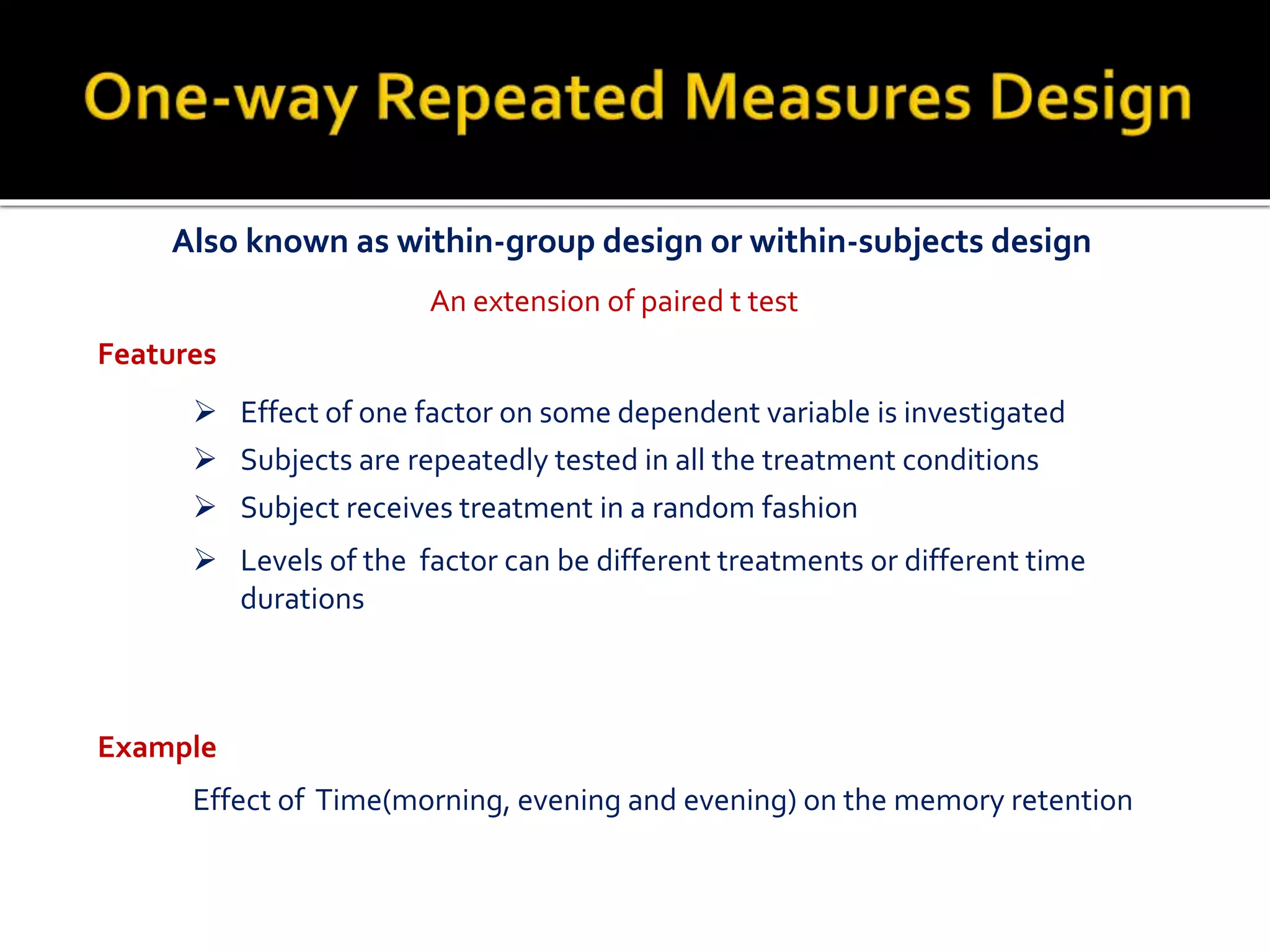
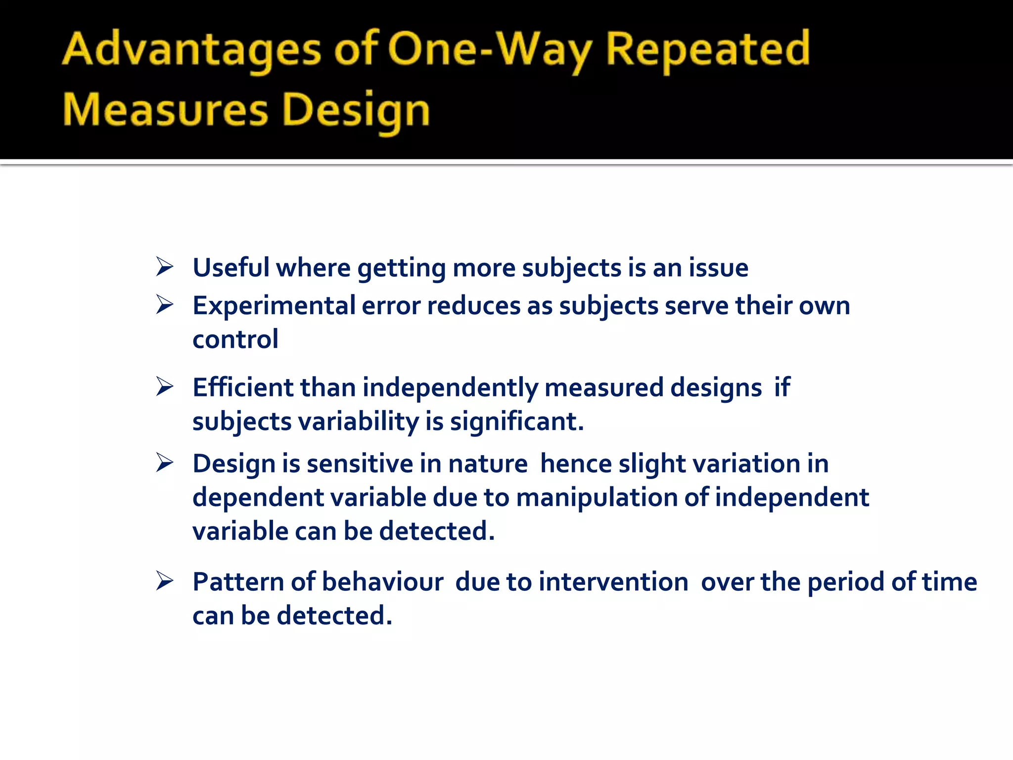
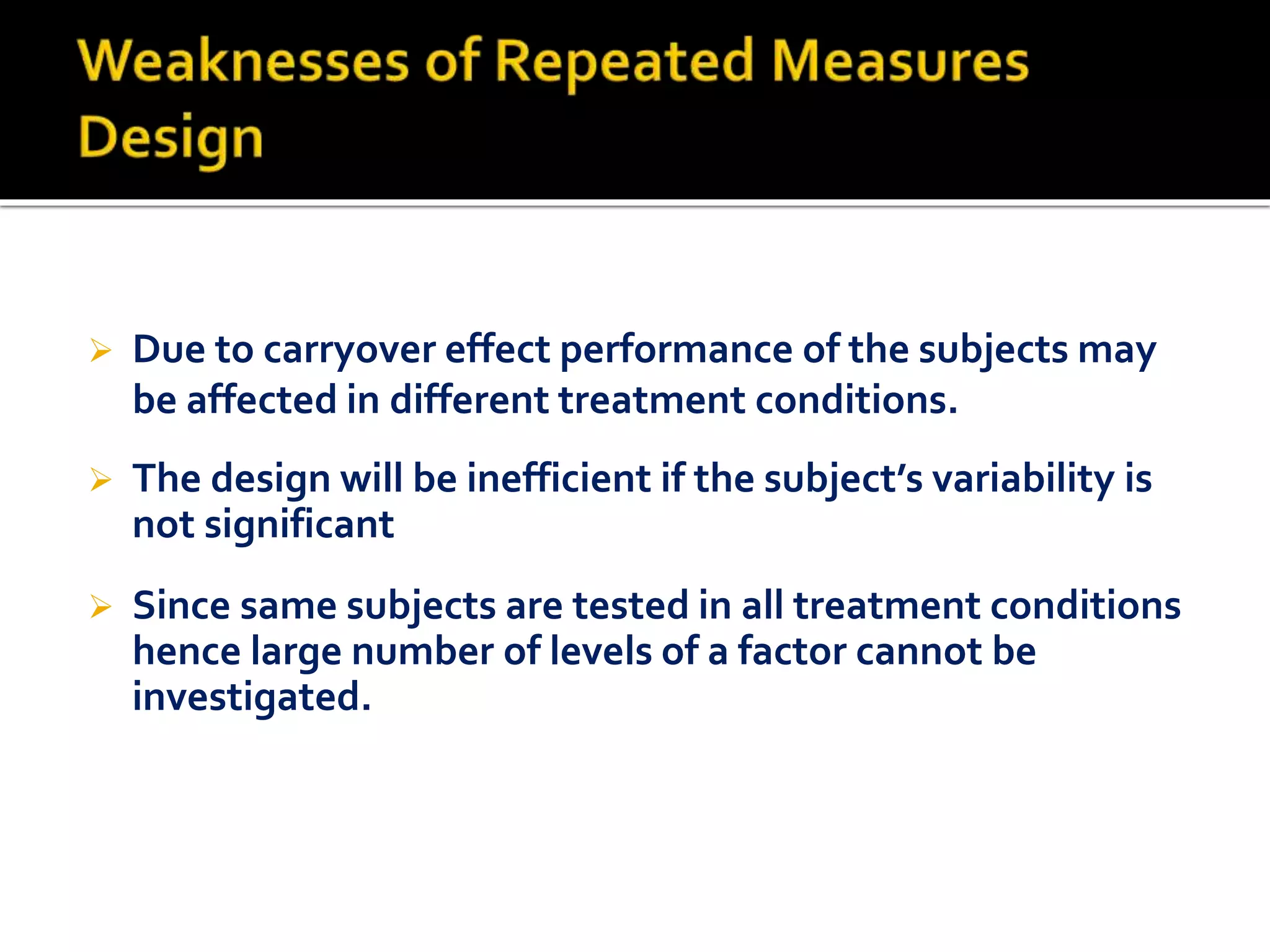
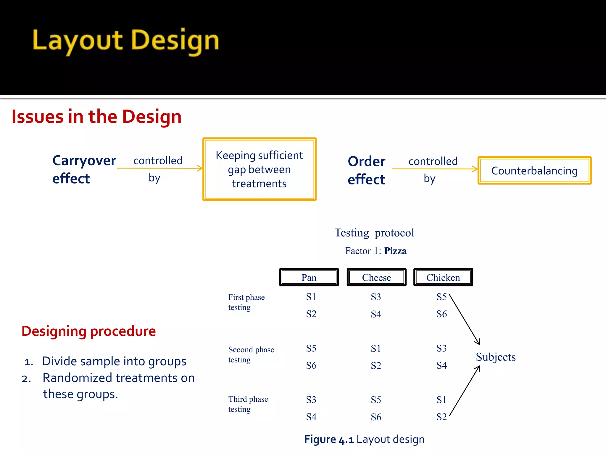
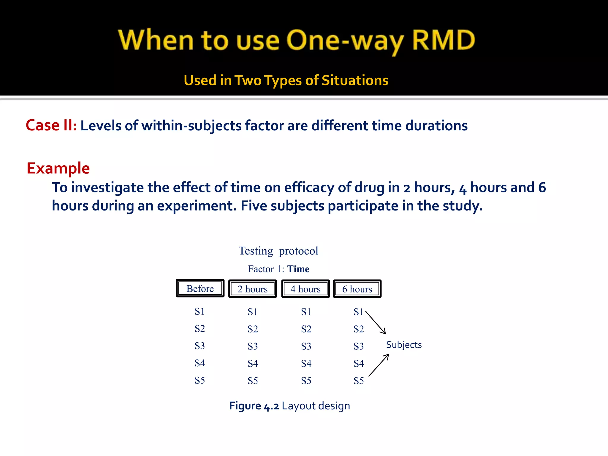
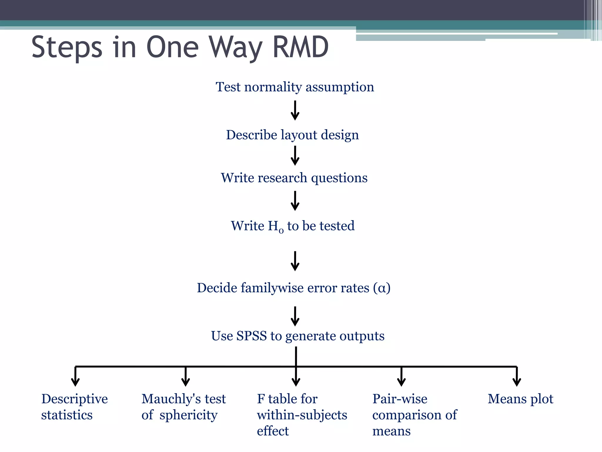
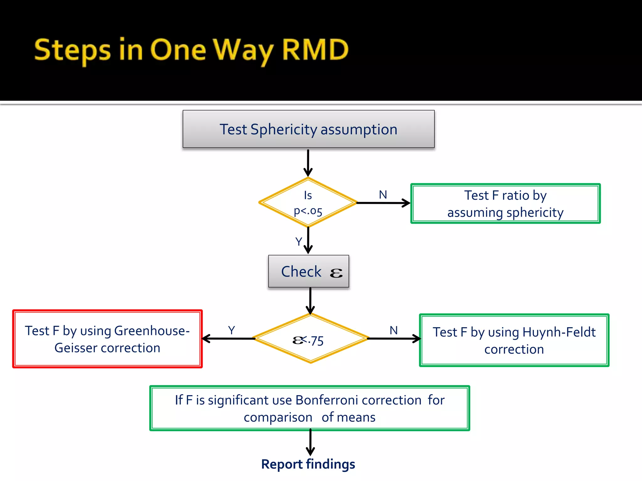
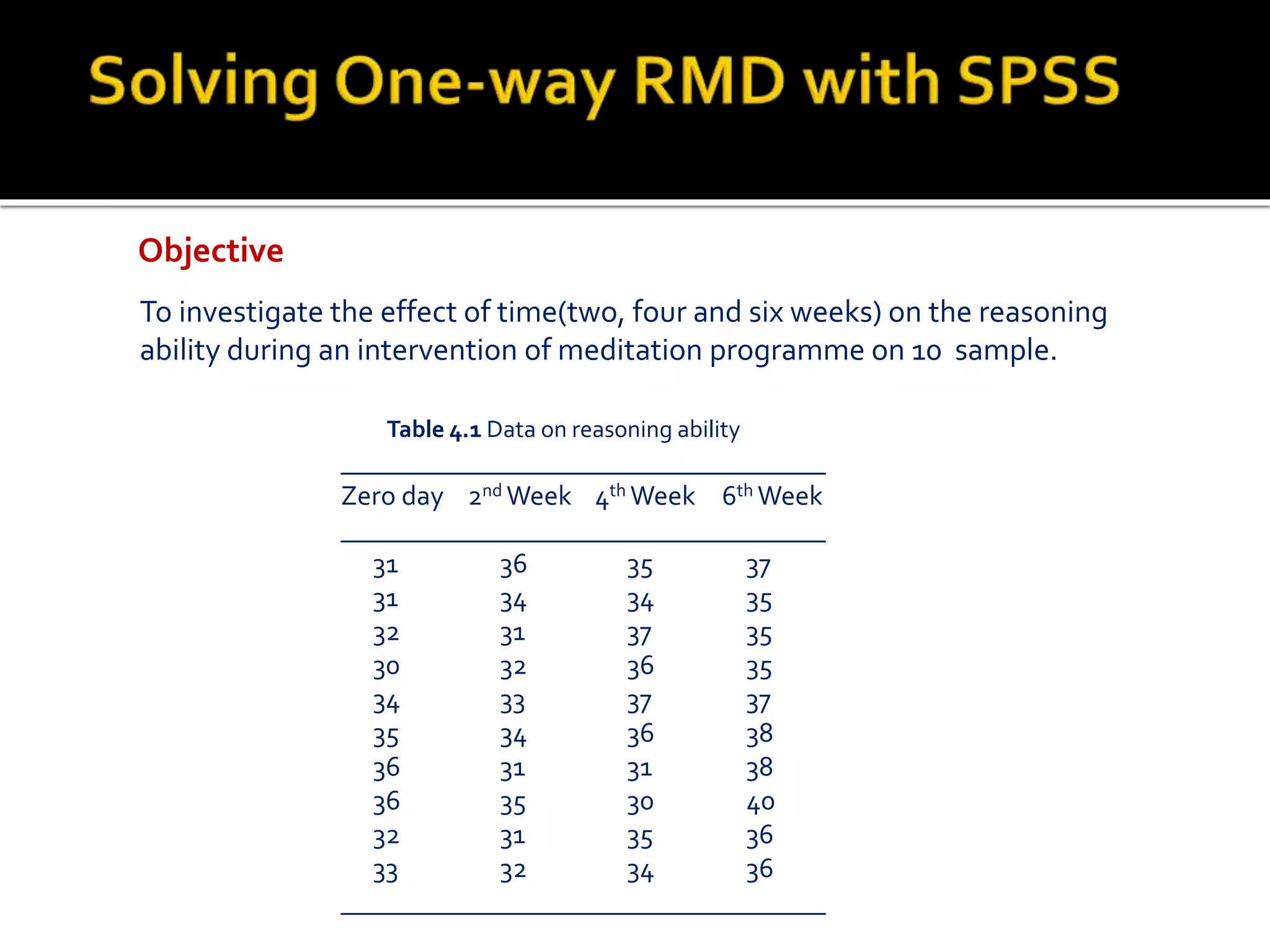
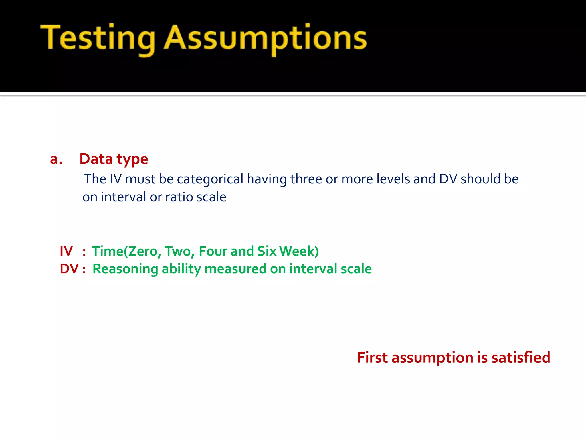
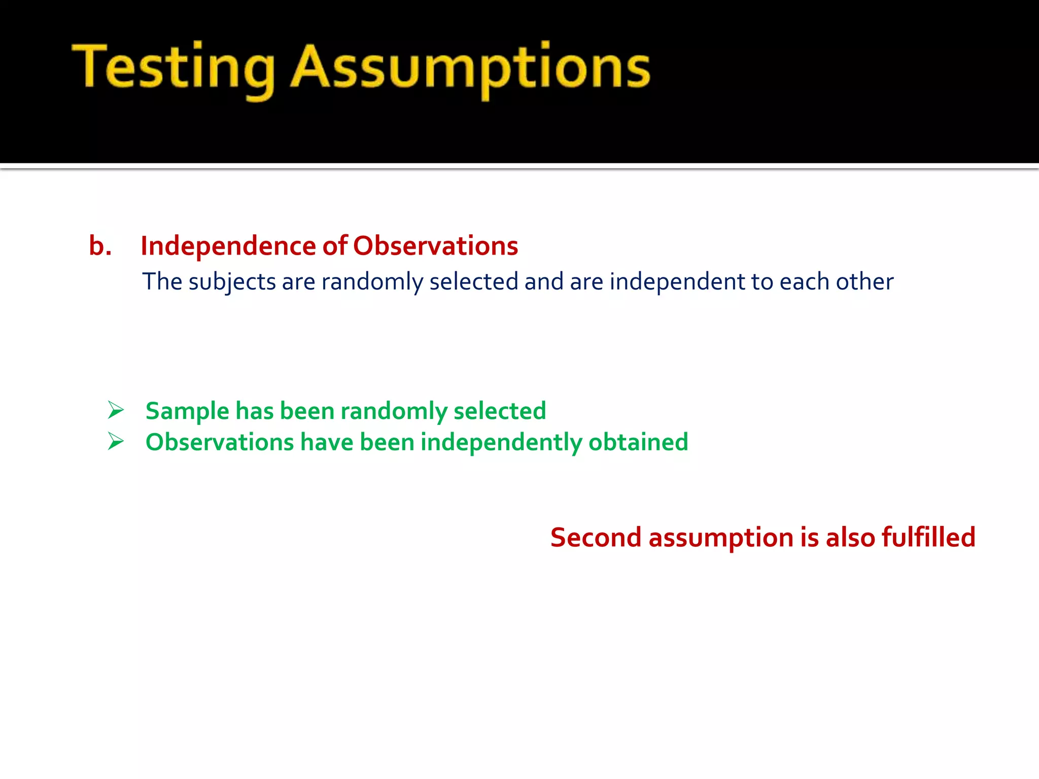
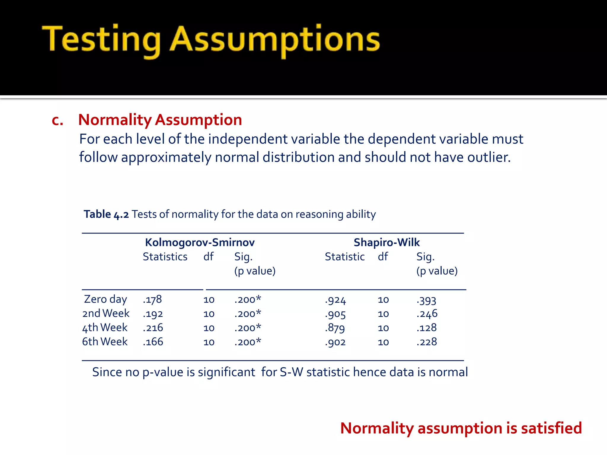
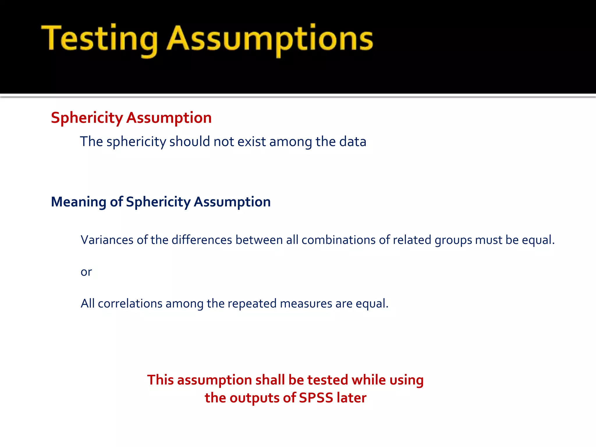
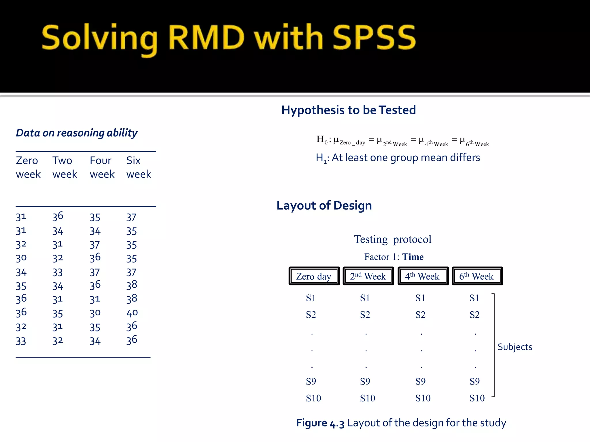
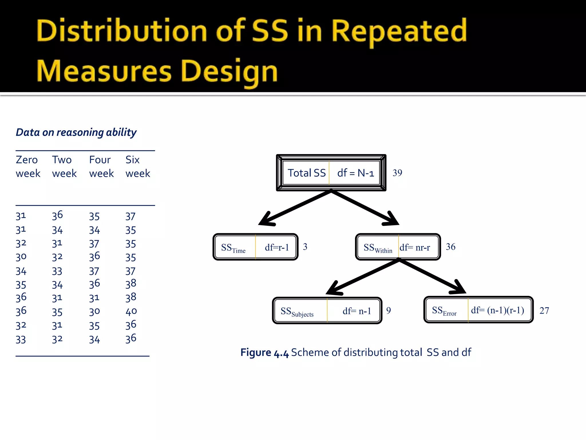
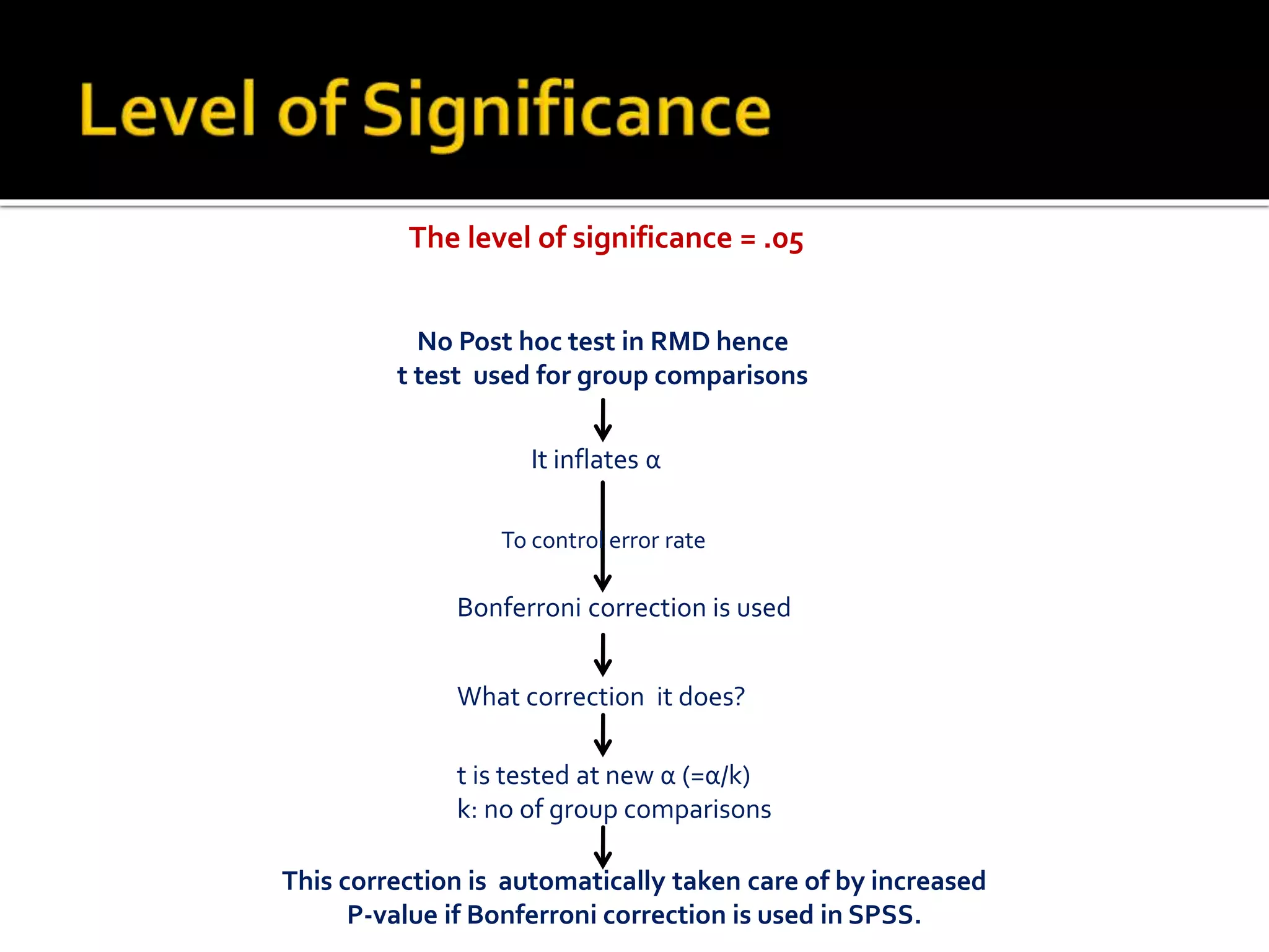
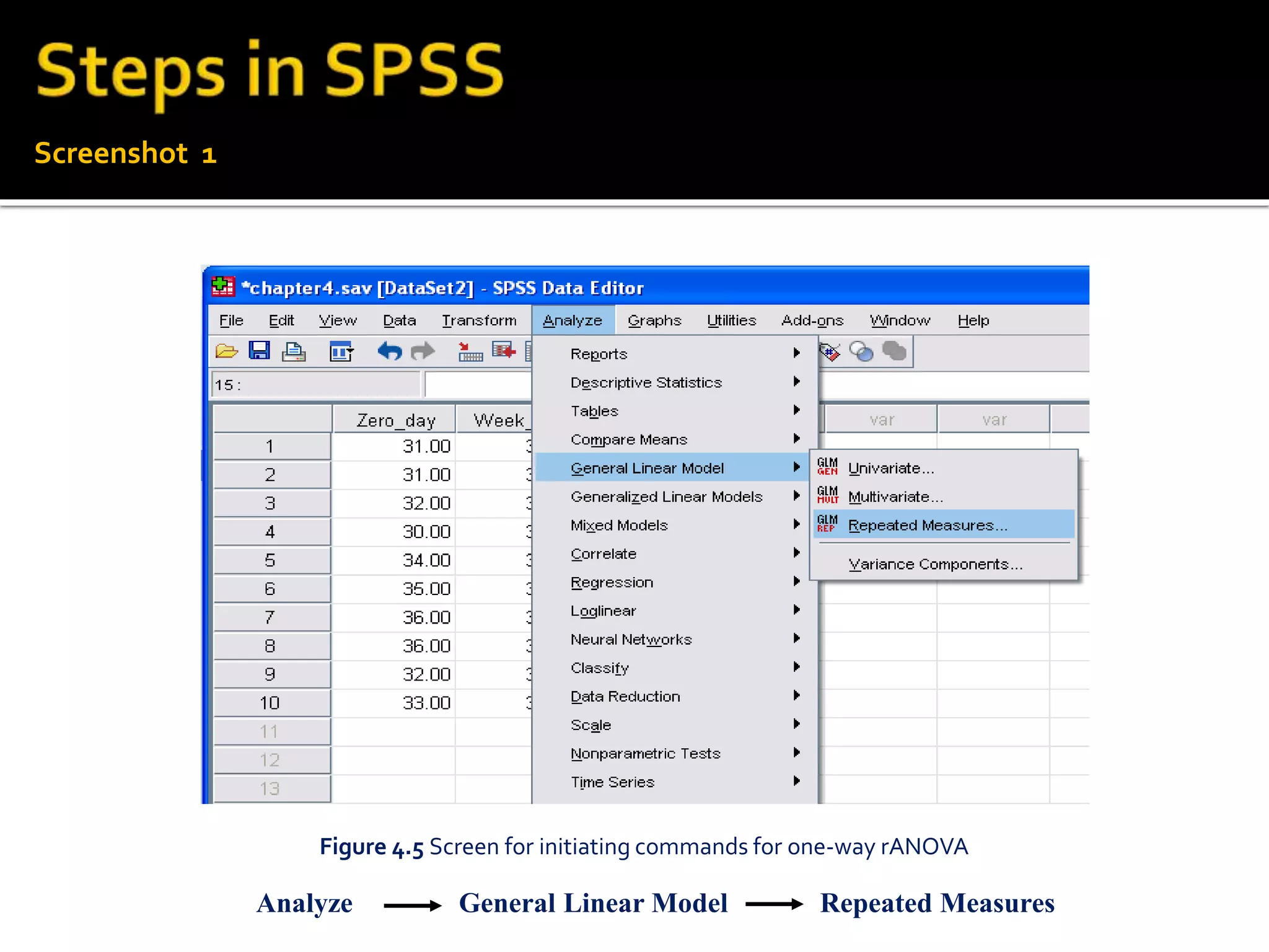
Presented by
Dr.J.P.Verma
MSc (Statistics), PhD, MA(Psychology), Masters(Computer Application)
Professor(Statistics)
Director, Centre for Advanced Studies
Lakshmibai National Institute of Physical Education, Gwalior, India
(Deemed University)
Email: vermajprakash@gmail.com
This Presentation is based on the book titled
Repeated Measures Designs for Empirical Researchers by Wiley USA
For Details Kindly click here
An extension of paired t test
Features
 Effect of one factor on some dependent variable is investigated
Example
Effect of Time(morning, evening and evening) on the memory retention
Also known as within-group design or within-subjects design
 Subjects are repeatedly tested in all the treatment conditions
 Subject receives treatment in a random fashion
 Levels of the factor can be different treatments or different time
durations
 Pattern of behaviour due to intervention over the period of time
can be detected.
 Useful where getting more subjects is an issue
 Experimental error reduces as subjects serve their own
control
 Efficient than independently measured designs if
subjects variability is significant.
 Design is sensitive in nature hence slight variation in
dependent variable due to manipulation of independent
variable can be detected.
 Due to carryover effect performance of the subjects may
be affected in different treatment conditions.
 Since same subjects are tested in all treatment conditions
hence large number of levels of a factor cannot be
investigated.
 The design will be inefficient if the subject’s variability is
not significant
This Presentation was based on the book titled Repeated Measures
Designs for Empirical Researchers by Wiley USA
For Details Kindly click here
 In a clinical experiment the drug efficacy can be tested by
taking hourly blood samples for 12 hours after its
administration.
 To compare recovery pattern of soccer players under light
exercise, autogenic relaxation and underwater exercise
 A physiologist may study an intervention of pranayama in
the relief of asthma
 Pizza company may investigate the taste of different types
of pizza on youngsters.
To compare the taste of different pizza in a specific age category of the
subjects. Six subjects participate in the study.
Example
Case I: Levels of within-subjects factor are different treatment conditions
Used inTwoTypes of Situations
Issues in the Design
Carryover
effect
controlled
by
Keeping sufficient
gap between
treatments
Order
effect
controlled
by
Counterbalancing
1. Divide sample into groups
2. Randomized treatments on
these groups.
Designing procedure
S1
S2
S5
S6
S3
S4
Factor 1: Pizza
S3
S4
S1
S2
S5
S6
S5
S6
S3
S4
S1
S2
Testing protocol
First phase
testing
Second phase
testing
Third phase
testing
ChickenPan Cheese
Subjects
Figure 4.1 Layout design
To investigate the effect of time on efficacy of drug in 2 hours, 4 hours and 6
hours during an experiment. Five subjects participate in the study.
Example
Case II: Levels of within-subjects factor are different time durations
Used inTwoTypes of Situations
2 hours
S1
S2
S3
S4
S5
S1
S2
S3
S4
S5
S1
S2
S3
S4
S5
4 hours 6 hours
Subjects
Before
S1
S2
S3
S4
S5
Factor 1: Time
Testing protocol
Figure 4.2 Layout design
Steps in One Way RMD
Test normality assumption
Describe layout design
Write research questions
Write H0 to be tested
Decide familywise error rates (α)
Use SPSS to generate outputs
Descriptive
statistics
Mauchly's test
of sphericity
F table for
within-subjects
effect
Pair-wise
comparison of
means
Means plot
Test Sphericity assumption
Is
p<.05
Test F ratio by
assuming sphericity
N
Y
Check 
<.75 Test F by using Huynh-Feldt
correction
NTest F by using Greenhouse-
Geisser correction
Y
If F is significant use Bonferroni correction for
comparison of means
Report findings
To investigate the effect of time(two, four and six weeks) on the reasoning
ability during an intervention of meditation programme on 10 sample.
Objective
Table 4.1 Data on reasoning ability
___________________________________
Zero day 2nd Week 4th Week 6th Week
___________________________________
31 36 35 37
31 34 34 35
32 31 37 35
30 32 36 35
34 33 37 37
35 34 36 38
36 31 31 38
36 35 30 40
32 31 35 36
33 32 34 36
___________________________________
a. Data type
The IV must be categorical having three or more levels and DV should be
on interval or ratio scale
IV : Time(Zero,Two, Four and Six Week)
DV : Reasoning ability measured on interval scale
First assumption is satisfied
 Sample has been randomly selected
 Observations have been independently obtained
Second assumption is also fulfilled
b. Independence of Observations
The subjects are randomly selected and are independent to each other
c. Normality Assumption
For each level of the independent variable the dependent variable must
follow approximately normal distribution and should not have outlier.
Table 4.2 Tests of normality for the data on reasoning ability
__________________________________________________________________
Kolmogorov-Smirnov Shapiro-Wilk
Statistics df Sig. Statistic df Sig.
(p value) (p value)
_____________________ _____________________________________________
Zero day .178 10 .200* .924 10 .393
2ndWeek .192 10 .200* .905 10 .246
4thWeek .216 10 .200* .879 10 .128
6thWeek .166 10 .200* .902 10 .228
__________________________________________________________________
Since no p-value is significant for S-W statistic hence data is normal
Normality assumption is satisfied
Sphericity Assumption
The sphericity should not exist among the data
Variances of the differences between all combinations of related groups must be equal.
or
All correlations among the repeated measures are equal.
Meaning of Sphericity Assumption
This assumption shall be tested while using
the outputs of SPSS later
Data on reasoning ability
_________________________
Zero Two Four Six
week week week week
_________________________
31 36 35 37
31 34 34 35
32 31 37 35
30 32 36 35
34 33 37 37
35 34 36 38
36 31 31 38
36 35 30 40
32 31 35 36
33 32 34 36
________________________
Layout of Design
Hypothesis to beTested
Factor 1: Time
Testing protocol
Subjects
Zero day
S1
S2
.
.
.
S9
S10
2nd Week 4th Week 6th Week
S1
S2
.
.
.
S9
S10
S1
S2
.
.
.
S9
S10
S1
S2
.
.
.
S9
S10
Week6Week4Week2day_Zero0 ththnd:H 
H1: At least one group mean differs
Figure 4.3 Layout of the design for the study
Data on reasoning ability
_________________________
Zero Two Four Six
week week week week
_________________________
31 36 35 37
31 34 34 35
32 31 37 35
30 32 36 35
34 33 37 37
35 34 36 38
36 31 31 38
36 35 30 40
32 31 35 36
33 32 34 36
________________________
SSTime df=r-1
Total SS df = N-1
SSWithin df= nr-r
39
3 36
SSError df= (n-1)(r-1)SSSubjects df= n-1 9 27
Figure 4.4 Scheme of distributing total SS and df
The level of significance = .05
No Post hoc test in RMD hence
t test used for group comparisons
It inflates α
To control error rate
Bonferroni correction is used
What correction it does?
t is tested at new α (=α/k)
k: no of group comparisons
This correction is automatically taken care of by increased
P-value if Bonferroni correction is used in SPSS.
Screenshot 1
Analyze General Linear Model Repeated Measures
Figure 4.5 Screen for initiating commands for one-way rANOVA
Screenshot 2
Figure 4.6 Options for defining dependent and independent variables
Screenshot 3
Write repeated
factor ‘Time’
Write levels of the
repeated factor ‘4’
and click onAdd
Write name of
the dependent
variable
Click on Add to define
this variables
Figure 4.7 Options for adding independent and dependent variables
1
2
3
4
Figure 4.8 Option for selecting within subjects
variables (Time) and obtaining means plot
Screenshot 4
Bring these variables
from left panel to this
location
Click on Plots
for means plot
Bring ‘Time’ factor at
this location
Click on
Continue
1
2
3
4
Screenshot 5
Figure 4.9 Option for descriptive statistics and pair wise
Comparison of means using Bonferroni correction
Click on Options
Bring ‘Time’ factor at
this location
Check these
options
1
2
3
4
 Descriptive Statistics
 Mauchly'sTest of Sphericity
 FTable for testing within-subjects effects
 Table for pair-wise comparison of means
 Marginal means plot
Output 1: Descriptive Statistics
Table 4.3 Descriptive statistics
_____________________________________
Mean SD N
_____________________________________
Zero_day 33.0000 2.16025 10
Week_two 32.9000 1.79196 10
Week_four 34.5000 2.36878 10
Week_six 36.7000 1.63639 10
_____________________________________
Output 2: Mauchly'sTest
Measure: Reasoning_ability Table 4.4 Mauchly's test of Sphericitya
_________________________________________________________________________________
Epsilona( )
Within Subjects Mauchly'sW Approx. Chi- df Sig. Greenhouse- Huynh- Lower-
Effect Square Geisser Feldt bound
_________________________________________________________________________________
Time .062 21.441 5 .001 .546 .650 .333
_________________________________________________________________________________
Assumption of Sphericity is violated because chi-square is significant

Table 4.5 F-Table for testing significance of Within-Subjects Effects
Measure: Reasoning_ability
_________________________________________________________________________________________
Source Type III df Mean Square F Sig. Partial
SS Eta Squared
_________________________________________________________________________________________
Time Sphericity Assumed 94.475 3 31.492 7.281 .001 .447
Greenhouse-Geisser 94.475 1.637 57.725 7.281 .009 .447
Huynh-Feldt 94.475 1.951 48.423 7.281 .005 .447
Lower-bound 94.475 1.000 94.475 7.281 .024 .447
Error(Time) Sphericity Assumed 116.775 27 4.325
Greenhouse-Geisser 116.775 14.730 7.928
Huynh-Feldt 116.775 17.559 6.650
Lower-bound 116.775 9.000 12.975
__________________________________________________________________________________________
Output 3: rANOVATable for testing within-subjects effects
Greenhouse Geisser: df forTreatment = ε × 2= 0.517 × 2= 1.03
df for Error = ε × 8 = 0.517 × 8 = = 4.14
Huynh- Feldt: df forTreatment = ε ×2 = 0.535 × 2 = 1.07
df for Error = ε × 8 = 0.535 × 8 = 4.28
Due to correction in degrees of freedom p values increases.
)1n)(1r(
SS
)1r(
SS
F
Error
Time



)1n)(1r(
SS
)1r(
SS
F
Error
Time



)1n)(1r(
SS
)1r(
SS
Error
Time



a. If sphericity is assumed

b. If sphericity exists the modified
degrees of freedom for SStime
and SSError gets modified by
multiplying them by
F remains same irrespective of the fact whether sphericity exists or not.
 After Greenhouse-Geisser correction the F is significant
p=.009(<.05)
 Partial Eta Square is .447, indicates very high effect size
The effect of time is meaningful to enhance reasoning
ability with meditation intervention.
Conclusion
What Next ?
Apply t test with Bonferroni correction for pair-wise
comparison of marginal means
Eta square
Value .02 .13 .26
Status Small Medium Large
Table 4.6 Pair wise Comparison of marginal means
Measure: Reasoning_ability
_____________________________________________________________________________
Mean Diff. 95% CI for Differencea
(I)Time (J)Time (I-J) Std. Error Siga Lower Bound Upper Bound
_____________________________________________________________________________
Zero_day Week_two .100 .875 1.000 -1.879 2.079
Week_four -1.500 1.267 1.000 -4.366 1.366
Week_six -3.700* .367 .000 -4.529 -2.871
Week_two Zero_day -.100 .875 1.000 -2.079 1.879
Week_four -1.600 1.013 .893 -3.892 .692
Week_six -3.800* .573 .001 -5.097 -2.503
Week_four Zero_day 1.500 1.267 1.000 -1.366 4.366
Week_two 1.600 1.013 .893 -.692 3.892
Week_six -2.200 1.153 .532 -4.808 .408
Week_six Zero_day 3.700* .367 .000 2.871 4.529
Week_two 3.800* .573 .001 2.503 5.097
Week_four 2.200 1.153 .532 -.408 4.808
_____________________________________________________________________________
Based on estimated marginal means
a. Adjustment for multiple comparisons: Bonferroni
*.The mean difference is significant at the .05 level.
Zero_day Week_two Week_four Week_six
Time
Estimatedmarginalmeansofreasoningability
Variable: Reasoning ability
Marginal means plot
 Meditation intervention program significantly affects the reasoning
ability of the subjects.
 The significant effect was observed only after the six weeks of the
intervention program.
Inference
Figure 4.10 Marginal means plot

Repeated measures anova with spss

  • 1.
    Presented by Dr.J.P.Verma MSc (Statistics),PhD, MA(Psychology), Masters(Computer Application) Professor(Statistics) Director, Centre for Advanced Studies Lakshmibai National Institute of Physical Education, Gwalior, India (Deemed University) Email: vermajprakash@gmail.com This Presentation is based on the book titled Repeated Measures Designs for Empirical Researchers by Wiley USA For Details Kindly click here
  • 2.
    An extension ofpaired t test Features  Effect of one factor on some dependent variable is investigated Example Effect of Time(morning, evening and evening) on the memory retention Also known as within-group design or within-subjects design  Subjects are repeatedly tested in all the treatment conditions  Subject receives treatment in a random fashion  Levels of the factor can be different treatments or different time durations
  • 3.
     Pattern ofbehaviour due to intervention over the period of time can be detected.  Useful where getting more subjects is an issue  Experimental error reduces as subjects serve their own control  Efficient than independently measured designs if subjects variability is significant.  Design is sensitive in nature hence slight variation in dependent variable due to manipulation of independent variable can be detected.
  • 4.
     Due tocarryover effect performance of the subjects may be affected in different treatment conditions.  Since same subjects are tested in all treatment conditions hence large number of levels of a factor cannot be investigated.  The design will be inefficient if the subject’s variability is not significant
  • 5.
    This Presentation wasbased on the book titled Repeated Measures Designs for Empirical Researchers by Wiley USA For Details Kindly click here
  • 6.
     In aclinical experiment the drug efficacy can be tested by taking hourly blood samples for 12 hours after its administration.  To compare recovery pattern of soccer players under light exercise, autogenic relaxation and underwater exercise  A physiologist may study an intervention of pranayama in the relief of asthma  Pizza company may investigate the taste of different types of pizza on youngsters.
  • 7.
    To compare thetaste of different pizza in a specific age category of the subjects. Six subjects participate in the study. Example Case I: Levels of within-subjects factor are different treatment conditions Used inTwoTypes of Situations
  • 8.
    Issues in theDesign Carryover effect controlled by Keeping sufficient gap between treatments Order effect controlled by Counterbalancing 1. Divide sample into groups 2. Randomized treatments on these groups. Designing procedure S1 S2 S5 S6 S3 S4 Factor 1: Pizza S3 S4 S1 S2 S5 S6 S5 S6 S3 S4 S1 S2 Testing protocol First phase testing Second phase testing Third phase testing ChickenPan Cheese Subjects Figure 4.1 Layout design
  • 9.
    To investigate theeffect of time on efficacy of drug in 2 hours, 4 hours and 6 hours during an experiment. Five subjects participate in the study. Example Case II: Levels of within-subjects factor are different time durations Used inTwoTypes of Situations 2 hours S1 S2 S3 S4 S5 S1 S2 S3 S4 S5 S1 S2 S3 S4 S5 4 hours 6 hours Subjects Before S1 S2 S3 S4 S5 Factor 1: Time Testing protocol Figure 4.2 Layout design
  • 10.
    Steps in OneWay RMD Test normality assumption Describe layout design Write research questions Write H0 to be tested Decide familywise error rates (α) Use SPSS to generate outputs Descriptive statistics Mauchly's test of sphericity F table for within-subjects effect Pair-wise comparison of means Means plot
  • 11.
    Test Sphericity assumption Is p<.05 TestF ratio by assuming sphericity N Y Check  <.75 Test F by using Huynh-Feldt correction NTest F by using Greenhouse- Geisser correction Y If F is significant use Bonferroni correction for comparison of means Report findings
  • 12.
    To investigate theeffect of time(two, four and six weeks) on the reasoning ability during an intervention of meditation programme on 10 sample. Objective Table 4.1 Data on reasoning ability ___________________________________ Zero day 2nd Week 4th Week 6th Week ___________________________________ 31 36 35 37 31 34 34 35 32 31 37 35 30 32 36 35 34 33 37 37 35 34 36 38 36 31 31 38 36 35 30 40 32 31 35 36 33 32 34 36 ___________________________________
  • 13.
    a. Data type TheIV must be categorical having three or more levels and DV should be on interval or ratio scale IV : Time(Zero,Two, Four and Six Week) DV : Reasoning ability measured on interval scale First assumption is satisfied
  • 14.
     Sample hasbeen randomly selected  Observations have been independently obtained Second assumption is also fulfilled b. Independence of Observations The subjects are randomly selected and are independent to each other
  • 15.
    c. Normality Assumption Foreach level of the independent variable the dependent variable must follow approximately normal distribution and should not have outlier. Table 4.2 Tests of normality for the data on reasoning ability __________________________________________________________________ Kolmogorov-Smirnov Shapiro-Wilk Statistics df Sig. Statistic df Sig. (p value) (p value) _____________________ _____________________________________________ Zero day .178 10 .200* .924 10 .393 2ndWeek .192 10 .200* .905 10 .246 4thWeek .216 10 .200* .879 10 .128 6thWeek .166 10 .200* .902 10 .228 __________________________________________________________________ Since no p-value is significant for S-W statistic hence data is normal Normality assumption is satisfied
  • 16.
    Sphericity Assumption The sphericityshould not exist among the data Variances of the differences between all combinations of related groups must be equal. or All correlations among the repeated measures are equal. Meaning of Sphericity Assumption This assumption shall be tested while using the outputs of SPSS later
  • 17.
    Data on reasoningability _________________________ Zero Two Four Six week week week week _________________________ 31 36 35 37 31 34 34 35 32 31 37 35 30 32 36 35 34 33 37 37 35 34 36 38 36 31 31 38 36 35 30 40 32 31 35 36 33 32 34 36 ________________________ Layout of Design Hypothesis to beTested Factor 1: Time Testing protocol Subjects Zero day S1 S2 . . . S9 S10 2nd Week 4th Week 6th Week S1 S2 . . . S9 S10 S1 S2 . . . S9 S10 S1 S2 . . . S9 S10 Week6Week4Week2day_Zero0 ththnd:H  H1: At least one group mean differs Figure 4.3 Layout of the design for the study
  • 18.
    Data on reasoningability _________________________ Zero Two Four Six week week week week _________________________ 31 36 35 37 31 34 34 35 32 31 37 35 30 32 36 35 34 33 37 37 35 34 36 38 36 31 31 38 36 35 30 40 32 31 35 36 33 32 34 36 ________________________ SSTime df=r-1 Total SS df = N-1 SSWithin df= nr-r 39 3 36 SSError df= (n-1)(r-1)SSSubjects df= n-1 9 27 Figure 4.4 Scheme of distributing total SS and df
  • 19.
    The level ofsignificance = .05 No Post hoc test in RMD hence t test used for group comparisons It inflates α To control error rate Bonferroni correction is used What correction it does? t is tested at new α (=α/k) k: no of group comparisons This correction is automatically taken care of by increased P-value if Bonferroni correction is used in SPSS.
  • 20.
    Screenshot 1 Analyze GeneralLinear Model Repeated Measures Figure 4.5 Screen for initiating commands for one-way rANOVA
  • 21.
    Screenshot 2 Figure 4.6Options for defining dependent and independent variables
  • 22.
    Screenshot 3 Write repeated factor‘Time’ Write levels of the repeated factor ‘4’ and click onAdd Write name of the dependent variable Click on Add to define this variables Figure 4.7 Options for adding independent and dependent variables 1 2 3 4
  • 23.
    Figure 4.8 Optionfor selecting within subjects variables (Time) and obtaining means plot Screenshot 4 Bring these variables from left panel to this location Click on Plots for means plot Bring ‘Time’ factor at this location Click on Continue 1 2 3 4
  • 24.
    Screenshot 5 Figure 4.9Option for descriptive statistics and pair wise Comparison of means using Bonferroni correction Click on Options Bring ‘Time’ factor at this location Check these options 1 2 3 4
  • 25.
     Descriptive Statistics Mauchly'sTest of Sphericity  FTable for testing within-subjects effects  Table for pair-wise comparison of means  Marginal means plot
  • 26.
    Output 1: DescriptiveStatistics Table 4.3 Descriptive statistics _____________________________________ Mean SD N _____________________________________ Zero_day 33.0000 2.16025 10 Week_two 32.9000 1.79196 10 Week_four 34.5000 2.36878 10 Week_six 36.7000 1.63639 10 _____________________________________
  • 27.
    Output 2: Mauchly'sTest Measure:Reasoning_ability Table 4.4 Mauchly's test of Sphericitya _________________________________________________________________________________ Epsilona( ) Within Subjects Mauchly'sW Approx. Chi- df Sig. Greenhouse- Huynh- Lower- Effect Square Geisser Feldt bound _________________________________________________________________________________ Time .062 21.441 5 .001 .546 .650 .333 _________________________________________________________________________________ Assumption of Sphericity is violated because chi-square is significant 
  • 28.
    Table 4.5 F-Tablefor testing significance of Within-Subjects Effects Measure: Reasoning_ability _________________________________________________________________________________________ Source Type III df Mean Square F Sig. Partial SS Eta Squared _________________________________________________________________________________________ Time Sphericity Assumed 94.475 3 31.492 7.281 .001 .447 Greenhouse-Geisser 94.475 1.637 57.725 7.281 .009 .447 Huynh-Feldt 94.475 1.951 48.423 7.281 .005 .447 Lower-bound 94.475 1.000 94.475 7.281 .024 .447 Error(Time) Sphericity Assumed 116.775 27 4.325 Greenhouse-Geisser 116.775 14.730 7.928 Huynh-Feldt 116.775 17.559 6.650 Lower-bound 116.775 9.000 12.975 __________________________________________________________________________________________ Output 3: rANOVATable for testing within-subjects effects
  • 29.
    Greenhouse Geisser: dfforTreatment = ε × 2= 0.517 × 2= 1.03 df for Error = ε × 8 = 0.517 × 8 = = 4.14 Huynh- Feldt: df forTreatment = ε ×2 = 0.535 × 2 = 1.07 df for Error = ε × 8 = 0.535 × 8 = 4.28 Due to correction in degrees of freedom p values increases. )1n)(1r( SS )1r( SS F Error Time    )1n)(1r( SS )1r( SS F Error Time    )1n)(1r( SS )1r( SS Error Time    a. If sphericity is assumed  b. If sphericity exists the modified degrees of freedom for SStime and SSError gets modified by multiplying them by F remains same irrespective of the fact whether sphericity exists or not.
  • 30.
     After Greenhouse-Geissercorrection the F is significant p=.009(<.05)  Partial Eta Square is .447, indicates very high effect size The effect of time is meaningful to enhance reasoning ability with meditation intervention. Conclusion What Next ? Apply t test with Bonferroni correction for pair-wise comparison of marginal means Eta square Value .02 .13 .26 Status Small Medium Large
  • 31.
    Table 4.6 Pairwise Comparison of marginal means Measure: Reasoning_ability _____________________________________________________________________________ Mean Diff. 95% CI for Differencea (I)Time (J)Time (I-J) Std. Error Siga Lower Bound Upper Bound _____________________________________________________________________________ Zero_day Week_two .100 .875 1.000 -1.879 2.079 Week_four -1.500 1.267 1.000 -4.366 1.366 Week_six -3.700* .367 .000 -4.529 -2.871 Week_two Zero_day -.100 .875 1.000 -2.079 1.879 Week_four -1.600 1.013 .893 -3.892 .692 Week_six -3.800* .573 .001 -5.097 -2.503 Week_four Zero_day 1.500 1.267 1.000 -1.366 4.366 Week_two 1.600 1.013 .893 -.692 3.892 Week_six -2.200 1.153 .532 -4.808 .408 Week_six Zero_day 3.700* .367 .000 2.871 4.529 Week_two 3.800* .573 .001 2.503 5.097 Week_four 2.200 1.153 .532 -.408 4.808 _____________________________________________________________________________ Based on estimated marginal means a. Adjustment for multiple comparisons: Bonferroni *.The mean difference is significant at the .05 level.
  • 32.
    Zero_day Week_two Week_fourWeek_six Time Estimatedmarginalmeansofreasoningability Variable: Reasoning ability Marginal means plot  Meditation intervention program significantly affects the reasoning ability of the subjects.  The significant effect was observed only after the six weeks of the intervention program. Inference Figure 4.10 Marginal means plot