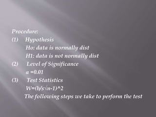
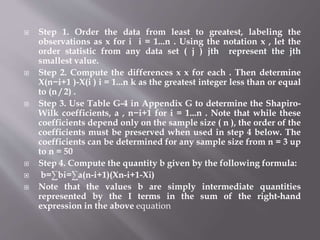
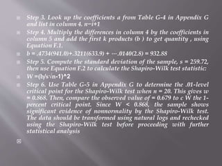
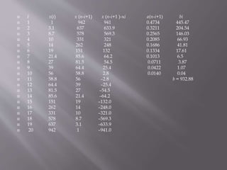
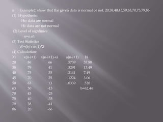
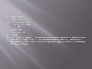
Shapiro Wilk Test
 The Shapiro–Wilk test is a test of normality in
frequentist statistics. It was published in 1965 by Samuel Sanford
Shapiro and Martin Wilk.
 Aussmption.
 The data is random
Samuel Sanford Shapiro
(born July 13, 1930) is an
American statistician and engineer. He is a professor emeritus of
statistics at Florida International University. He is known for his
co-authorship of the Shapiro–Wilk test. A native of New York
City, Shapiro graduated from City College of New York with a
degree in statistics in 1952, and took an MS in industrial
engineering at Columbia University in 1954. He briefly served
as a statistician in the US Army Chemical Corps, before earning
a MS (1960) and PhD (1963) in statistics at Rutgers
University. In 1972 he joined the faculty at Florida International
University
 Martin Bradbury Wilk,
 OC (18 December 1922 – 19 February 2013) was
a Canadian statistician, academic, and the former Chief
Statistician of Canada. In 1965, together with Samuel Shapiro,
he developed the Shapiro–Wilk test, which can indicate whether
a sample of numbers would be unusual if it came from
a Gaussian distribution. With Ramanathan Gnanadesikan he
developed a number of important graphical techniques for data
analysis, including the Q–Q plot and P–P plot.
 Born in Montréal, Québec, he received a Bachelor of
Engineering degree in Chemical Engineering from McGill
University in 1945. From 1945 to 1950, he was a Research
Chemical Engineer on the Atomic Energy Project at the National
Research Council of Canada. From 1951 to 1955, he was a
Research Associate, Instructor, and Assistant Professor at Iowa
State University, where he received a Master of Science in
Statistics in 1953 and a Ph.D. in Statistics in 1955. From 1955 to
1957, he was a Research Associate and Assistant Director of the
Statistical Techniques Research Group at Princeton University.
 . From 1959 to 1963, he was a Professor and Director of Research
in Statistics at Rutgers University In 1956, he joined Bell
Telephone Laboratories and in 1970 joined American Telephone
and Telegraph Company. From 1976 to 1980, he was the
Assistant Vice President-Director of Corporate Planning. From
1980 to 1985, he was the Chief Statistician of Canada. In 1981, he
was appointed an Adjunct Professor of Statistics at Carleton
University. In 1999, he was made an Officer of the Order of
Canada for his "insightful guidance on important matters
related to our country's national statistical system
Procedure:
(1) Hypothesis
Ho: data is normally dist
H1: data is not normally dist
(2) Level of Significance
α =0.01
(3) Test Statistics
W=(b/s√n-1)^2
The following steps we take to perform the test
 Step 1. Order the data from least to greatest, labeling the
observations as x for i i = 1...n . Using the notation x , let the
order statistic from any data set ( j ) jth represent the jth
smallest value.
 Step 2. Compute the differences x x for each . Then determine
X(n−i+1 )-X(i ) i = 1...n k as the greatest integer less than or equal
to (n / 2) .
 Step 3. Use Table G-4 in Appendix G to determine the Shapiro-
Wilk coefficients, a , n−i+1 for i = 1...n . Note that while these
coefficients depend only on the sample size ( n ), the order of the
coefficients must be preserved when used in step 4 below. The
coefficients can be determined for any sample size from n = 3 up
to n = 50
 Step 4. Compute the quantity b given by the following formula:
 b=∑bi=∑a(n-i+1)(Xn-i+1-Xi)
 Note that the values b are simply intermediate quantities
represented by the I terms in the sum of the right-hand
expression in the above equation
 Step 5. Calculate the standard deviation (s) of the data set. Then
compute the Shapiro-Wilk test statistic using the following
formula:
W=(b/s√n-1)^2
 Critical region and conclusion:
Given the significance level (α ) of the test (for
example, 0.01 or 0.05), determine the critical point of the Shapiro-
Wilk test with n observations using Table G-5 in Appendix G.
Compare the Shapiro-Wilk statistic (W) against the critical point (
w ). If the test statistic exceeds the critical point, accept normality c
as a reasonable model for the underlying population; however, if
W w , reject c < the null hypothesis of normality at the α -level and
decide that another distributional model would provide a better
fit.
 Example Calculation of the Shapiro-Wilk Test for Normality
 Use the Shapiro-Wilk test for normality to determine whether the
following data set, representing the total concentration of nickel
in a solid waste, follows a normal distribution: 58.8, 19, 39, 3.1, 1,
81.5, 151, 942, 262,331, 27, 85.6, 56, 14, 21.4, 10, 8.7, 64.4, 578, and
637.
 Solution
 Step 1. Order the data from smallest to largest and list, as in
Table F-2. Also list the data in reverse order alongside the first
column.
 Step 2. Compute the differences x x in column 4 of the table by
subtracting column 2 (n−i+ ) (i ) − 1 from column 3. Because the
total number of samples is n = 20 , the largest integer less than or
equal to (n / 2) is k = 10 .
 Step 3. Look up the coefficients a from Table G-4 in Appendix G
and list in column 4. n−i+1
 Step 4. Multiply the differences in column 4 by the coefficients in
column 5 and add the first k products (b ) to get quantity , using
Equation F.1.
 b = .4734(941.0)+.3211(633.9) + ⋅⋅⋅ .0140(2.8) = 932.88
 Step 5. Compute the standard deviation of the sample, s = 259.72,
then use Equation F.2 to calculate the Shapiro-Wilk test statistic:
 W =(b/s√n-1)^2
 Step 6. Use Table G-5 in Appendix G to determine the .01-level
critical point for the Shapiro-Wilk test when n = 20. This gives w
= 0.868. Then, compare the observed value of = 0.679 to c W the 1-
percent critical point. Since W < 0.868, the sample shows
significant evidence of nonnormality by the Shapiro-Wilk test.
The data should be transformed using natural logs and rechecked
using the Shapiro-Wilk test before proceeding with further
statistical analysis

 I x(i) x (n-i+1) x (n-i+1 )-xi a(n-i+1) bi
 1 1 942 941 0.4734 445.47
 2 3.1 637 633.9 0.3211 204.54
 3 8.7 578 569.3 0.2565 146.03
 4 10 331 321 0.2085 66.93
 5 14 262 248 0.1686 41.81
 6 19 151 132 0.1334 17.61
 7 21.4 85.6 64.2 0.1013 6.5
 8 27 81.5 54.5 0.0711 3.87
 9 39 64.4 25.4 0.0422 1.07
 10 56 58.8 2.8 0.0140 0.04
 11 58.8 56 –2.8 b = 932.88
 12 64.4 39 –25.4
 13 81.5 27 –54.5
 14 85.6 21.4 –64.2
 15 151 19 –132.0
 16 262 14 –248.0
 17 331 10 –321.0
 18 578 8.7 –569.3
 19 637 3.1 –633.9
 20 942 1 –941.0
 Example2: show that the given data is normal or not. 20,38,40,45,50,63,70,75,79,86
(1) Hypothesis;
Ho: data are normal
Hi: data are not normal
(2) Level of signfinice
α=o.o1
(3) Test Statistics
W=(b/s√n-1)^2
(4) Calaulation:
Xi x(n-i+1) x(n-i+1)-xi a(n-i+1) bi
20 86 66 .5739 37.88
38 79 41 .3291 13.49
40 75 35 .2141 7.49
45 70 25 .1224 3.06
50 63 13 .0339 .520
63 50 -13 b=62.44
70 45 -25
75 40 -35
79 38 -41
86 20 -66
 W=(b/s√n-1)^2
b= 62.44, n=10,s=20.16
put In above formula we get
=(62.44/20.16√10-1)^2
= 1.o66
(5) Critical region:
w(0.01)10= .781
(6) decision
 Use Table G-5 in Appendix G to determine the .01-level critical point for the Shapiro-Wilk test
when n = 10. This gives w = .781. Then, compare the observed value of = .1.066 to c W the 1-
percent critical point. Since W < 0.781, the sample shows significant evidence of normality by
the Shapiro-Wilk test.
 i  n 2 3 4 5 6 7 8 9 10
 1 .7071 .7071 .6872 .6646 .6431 .6233 .6052 .5888 .5739
 2 .0000 .1677 .2413 .2806 .3031 .3164 .3244 .3291
 3 .0000 .0875 .1401 .1743 .1976 .2141
 4 .0000 .0561 .0947 .1224
 5 .0000 .0399
 i  n 11 12 13 14 15 16 17 18 19 20
 1 .5601 .5475 .5359 .5251 .5150 .5056 .4968 .4886 .4808 .4734
 2 .3315 .3325 .3325 .3318 .3306 .3290 .3273 .3253 .3232 .3211
 3 .2260 .2347 .2412 .2460 .2495 .2521 .2540 .2553 .2561 .2565
 4 .1429 .1586 .1707 .1802 .1878 .1939 .1988 .2027 .2059 .2085
 5 .0695 .0922 .1099 .1240 .1353 .1447 .1524 .1587 .1641 .1686
 6 .0000 .0303 .0539 .0727 .0880 .1005 .1109 .1197 .1271 .1334
 7 .0000 .0240 .0433 .0593 .0725 .0837 .0932 .1013
 8 .0000 .0196 .0359 .0496 .0612 .0711
 9 .0000 .0163 .0303 .0422
 10 .0000 .0140
 i  n 21 22 23 24 25 26 27 28 29 30
1 .4643 .4590 .4542 .4493 .4450 .4407 .4366 .4328 .4291 .4254
2 .3185 .3156 .3126 .3098 .3069 .3043 .3018 .2992 .2968 .2944
3 .2578 .2571 .2563 .2554 .2543 .2533 .2522 .2510 .2499 .2487
4 .2119 .2131 .2139 .2145 .2148 .2151 .2152 .2151 .2150 .2148
5 .1736 .1764 .1787 .1807 .1822 .1836 .1848 .1857 .1864 .1870
6 .1399 .1443 .1480 .1512 .1539 .1563 .1584 .1601 .1616 .1630
7 .1092 .1150 .1201 .1245 .1283 .1316 .1346 .1372 .1395 .1415
8 .0804 .0878 .0941 .0997 .1046 .1089 .1128 .1162 .1192 .1219
9 .0530 .0618 .0696 .0764 .0823 .0876 .0923 .0965 .1002 .1036
10 .0263 .0368 .0459 .0539 .0610 .0672 .0728 .0778 .0822 .0862
11 .0000 .0228 .0321 .0403 .0476 .0540 .0598 .0650 .0697
12 .0000 .0107 .0200 .0284 .0358 .0424 .0483 .0537
13 .0000 .0094 .0178 .0253 .0320 .0367
14 .0000 .0084 .0159 .0227
 i  n 31 32 33 34 35 36 37 38 39 40
 1 .4220 .4188 .4156 .4127 .4096 .4068 .4040 .4015 .3989 .3964
 2 .2921 .2898 .2876 .2854 .2834 .2813 .2794 .2774 .2755 .2737
 3 .2475 .2463 .2451 .2439 .2427 .2415 .2403 .2391 .2380 .2368
 4 .2145 .2141 .2137 .2132 .2127 .2121 .2116 .2110 .2104 .2098
 5 .1874 .1878 .1880 .1882 .1883 .1883 .1883 .1881 .1880 .1878
 6 .1641 .1651 .1660 .1667 .1673 .1678 .1683 .1686 .1689 .1691
 7 .1433 .1449 .1463 .1475 .1487 .1496 .1505 .1513 .1520 .1526
 8 .1243 .1265 .1284 .1301 .1317 .1331 .1344 .1356 .1366 .1376
 9 .1066 .1093 .1118 .1140 .1160 .1179 .1196 .1211 .1225 .1237
 10 .0899 .0931 .0961 .0988 .1013 .1036 .1056 .1075 .1092 .1108
 11 .0739 .0777 .0812 .0844 .0873 .0900 .0924 .0947 .0967 .0986
 12 .0585 .0629 .0669 .0706 .0739 .0770 .0798 .0824 .0848 .0870
 13 .0435 .0485 .0530 .0572 .0610 .0645 .0677 .0706 .0733 .0759
 14 .0289 .0344 .0395 .0441 .0484 .0523 .0559 .0592 .0622 .0651
 15 .0144 .0206 .0262 .0314 .0361 .0404 .0444 .0481 .0515 .0546
 16 .0000 .0068 .0131 .0187 .0239 .0287 .0331 .0372 .0409 .0444
 17 .0000 .0062 .0119 .0172 .0220 .0264 .0305 .0343
 18 .0000 .0057 .0110 .0158 .0203 .0244
 19 .0000 .0053 .0101 .0146
 20 .0000 .0049
 i  n 41 42 43 44 45 46 47 48 49 50
 1 .3940 .3917 .3894 .3872 .3850 .3830 .3808 .3789 .3770 .3751
 2 .2719 .2701 .2628 .2667 .2651 .2635 .2620 .2604 .2589 .2574
 3 .2357 .2345 .2334 .2323 .2313 .2302 .2291 .2281 .2271 .2260
 4 .2091 .2085 .2078 .2072 .2065 .2058 .2052 .2045 .2038 .2032
 5 .1876 . 1874 .1871 .1868 .1865 .1862 .1859 .1855 .1851 .1847
 6 .1693 .1694 .1695 .1695 .1695 .1695 .1695 .1693 .1692 .1691
 7 .1531 .1535 .1539 .1542 .1545 .1548 .1550 .1551 .1553 .1554
 8 .1384 .1392 .1398 .1405 .1410 .1415 .1420 .1423 .1427 .1430
 9 .1249 .1259 .1269 .1278 .1286 .1293 .1300 .1306 .1312 .1317
 10 .1123 .1136 .1149 .1160 .1170 .1180 .1189 .1197 .1205 .1212
 11 .1004 .1020 .1035 .1049 .1062 .1073 .1085 .1095 .1105 .1113
 12 .0891 .0909 .0927 .0943 .0959 .0972 .0986 .0998 .1010 .1020
 13 .0782 .0804 .0824 .0842 .0860 .0876 .0892 .0906 .0919 .0932
 14 .0677 .0701 .0724 .0745 .0775 .0785 .0801 .0817 .0832 .0846
 15 .0575 .0602 .0628 .0651 .0673 .0694 .0713 .0731 .0748 .0764
 16 .0476 .0506 .0534 .0560 .0584 .0607 .0628 .0648 .0667 .0685
 17 .0379 .0411 .0442 .0471 .0497 .0522 .0546 .0568 .0588 .0608
 18 .0283 .0318 .0352 .0383 .0412 .0439 .0465 .0489 .0511 .0532
 19 .0188 .0227 .0263 .0296 .0328 .0357 .0385 .0411 .0436 .0459
 20 .0094 .0136 .0175 .0211 .0245 .0277 .0307 .0335 .0361 .0386
 21 .0000 .0045 .0087 .0126 .0163 .0197 .0229 .0259 .0288 .0314
 22 .0000 .0042 .0081 .0118 .0153 .0185 .0215 .0244
 23 .0000 .0039 .0076 .0111 .0143 .0174
 24 .0000 .0037 .0071 .0104
 25 .0000 .0035
 Table. -Level Critical Points for the Shapiro-Wilk Test



n 0.01 0.05
 3 0.753 0.767
 4 0.687 0.748
 5 0.686 0.762
 6 0.713 0.788
 7 0.730 0.803
 8 0.749 0.818
 9 0.764 0.829
 10 0.781 0.842
 11 0.792 0.850
 12 0.805 0.859
 13 0.814 0.866
 14 0.825 0.874
 15 0.835 0.881
 16 0.844 0.887
 17 0.851 0.892
 18 0.858 0.897
 19 0.863 0.901
 20 0.868 0.905
 21 0.873 0.908
 22 0.878 0.911
 23 0.881 0.914
 24 0.884 0.916
 25 0.888 0.918
 26 0.891 0.920
 27 0.894 0.923
 28 0.896 0.924
 29 0.898 0.926
 30 0.900 0.927
 31 0.902 0.929
 32 0.904 0.930
 33 0.906 0.931
 34 0.908 0.933
 35 0.910 0.934
 36 0.912 0.935
 37 0.914 0.936
 38 0.916 0.938
 39 0.917 0.939
 40 0.919 0.940
 41 0.920 0.941
 42 0.922 0.942
 43 0.923 0.943
 44 0.924 0.944
 45 0.926 0.945
 46 0.927 0.945
 47 0.928 0.946
 48 0.929 0.947
 49 0.929 0.947
 50 0.930 0.947

Shapiro wilk test

  • 2.
  • 3.
     The Shapiro–Wilktest is a test of normality in frequentist statistics. It was published in 1965 by Samuel Sanford Shapiro and Martin Wilk.  Aussmption.  The data is random
  • 4.
    Samuel Sanford Shapiro (bornJuly 13, 1930) is an American statistician and engineer. He is a professor emeritus of statistics at Florida International University. He is known for his co-authorship of the Shapiro–Wilk test. A native of New York City, Shapiro graduated from City College of New York with a degree in statistics in 1952, and took an MS in industrial engineering at Columbia University in 1954. He briefly served as a statistician in the US Army Chemical Corps, before earning a MS (1960) and PhD (1963) in statistics at Rutgers University. In 1972 he joined the faculty at Florida International University
  • 5.
     Martin BradburyWilk,  OC (18 December 1922 – 19 February 2013) was a Canadian statistician, academic, and the former Chief Statistician of Canada. In 1965, together with Samuel Shapiro, he developed the Shapiro–Wilk test, which can indicate whether a sample of numbers would be unusual if it came from a Gaussian distribution. With Ramanathan Gnanadesikan he developed a number of important graphical techniques for data analysis, including the Q–Q plot and P–P plot.  Born in Montréal, Québec, he received a Bachelor of Engineering degree in Chemical Engineering from McGill University in 1945. From 1945 to 1950, he was a Research Chemical Engineer on the Atomic Energy Project at the National Research Council of Canada. From 1951 to 1955, he was a Research Associate, Instructor, and Assistant Professor at Iowa State University, where he received a Master of Science in Statistics in 1953 and a Ph.D. in Statistics in 1955. From 1955 to 1957, he was a Research Associate and Assistant Director of the Statistical Techniques Research Group at Princeton University.
  • 6.
     . From1959 to 1963, he was a Professor and Director of Research in Statistics at Rutgers University In 1956, he joined Bell Telephone Laboratories and in 1970 joined American Telephone and Telegraph Company. From 1976 to 1980, he was the Assistant Vice President-Director of Corporate Planning. From 1980 to 1985, he was the Chief Statistician of Canada. In 1981, he was appointed an Adjunct Professor of Statistics at Carleton University. In 1999, he was made an Officer of the Order of Canada for his "insightful guidance on important matters related to our country's national statistical system
  • 7.
    Procedure: (1) Hypothesis Ho: datais normally dist H1: data is not normally dist (2) Level of Significance α =0.01 (3) Test Statistics W=(b/s√n-1)^2 The following steps we take to perform the test
  • 8.
     Step 1.Order the data from least to greatest, labeling the observations as x for i i = 1...n . Using the notation x , let the order statistic from any data set ( j ) jth represent the jth smallest value.  Step 2. Compute the differences x x for each . Then determine X(n−i+1 )-X(i ) i = 1...n k as the greatest integer less than or equal to (n / 2) .  Step 3. Use Table G-4 in Appendix G to determine the Shapiro- Wilk coefficients, a , n−i+1 for i = 1...n . Note that while these coefficients depend only on the sample size ( n ), the order of the coefficients must be preserved when used in step 4 below. The coefficients can be determined for any sample size from n = 3 up to n = 50  Step 4. Compute the quantity b given by the following formula:  b=∑bi=∑a(n-i+1)(Xn-i+1-Xi)  Note that the values b are simply intermediate quantities represented by the I terms in the sum of the right-hand expression in the above equation
  • 9.
     Step 5.Calculate the standard deviation (s) of the data set. Then compute the Shapiro-Wilk test statistic using the following formula: W=(b/s√n-1)^2  Critical region and conclusion: Given the significance level (α ) of the test (for example, 0.01 or 0.05), determine the critical point of the Shapiro- Wilk test with n observations using Table G-5 in Appendix G. Compare the Shapiro-Wilk statistic (W) against the critical point ( w ). If the test statistic exceeds the critical point, accept normality c as a reasonable model for the underlying population; however, if W w , reject c < the null hypothesis of normality at the α -level and decide that another distributional model would provide a better fit.
  • 10.
     Example Calculationof the Shapiro-Wilk Test for Normality  Use the Shapiro-Wilk test for normality to determine whether the following data set, representing the total concentration of nickel in a solid waste, follows a normal distribution: 58.8, 19, 39, 3.1, 1, 81.5, 151, 942, 262,331, 27, 85.6, 56, 14, 21.4, 10, 8.7, 64.4, 578, and 637.  Solution  Step 1. Order the data from smallest to largest and list, as in Table F-2. Also list the data in reverse order alongside the first column.  Step 2. Compute the differences x x in column 4 of the table by subtracting column 2 (n−i+ ) (i ) − 1 from column 3. Because the total number of samples is n = 20 , the largest integer less than or equal to (n / 2) is k = 10 .
  • 11.
     Step 3.Look up the coefficients a from Table G-4 in Appendix G and list in column 4. n−i+1  Step 4. Multiply the differences in column 4 by the coefficients in column 5 and add the first k products (b ) to get quantity , using Equation F.1.  b = .4734(941.0)+.3211(633.9) + ⋅⋅⋅ .0140(2.8) = 932.88  Step 5. Compute the standard deviation of the sample, s = 259.72, then use Equation F.2 to calculate the Shapiro-Wilk test statistic:  W =(b/s√n-1)^2  Step 6. Use Table G-5 in Appendix G to determine the .01-level critical point for the Shapiro-Wilk test when n = 20. This gives w = 0.868. Then, compare the observed value of = 0.679 to c W the 1- percent critical point. Since W < 0.868, the sample shows significant evidence of nonnormality by the Shapiro-Wilk test. The data should be transformed using natural logs and rechecked using the Shapiro-Wilk test before proceeding with further statistical analysis 
  • 12.
     I x(i)x (n-i+1) x (n-i+1 )-xi a(n-i+1) bi  1 1 942 941 0.4734 445.47  2 3.1 637 633.9 0.3211 204.54  3 8.7 578 569.3 0.2565 146.03  4 10 331 321 0.2085 66.93  5 14 262 248 0.1686 41.81  6 19 151 132 0.1334 17.61  7 21.4 85.6 64.2 0.1013 6.5  8 27 81.5 54.5 0.0711 3.87  9 39 64.4 25.4 0.0422 1.07  10 56 58.8 2.8 0.0140 0.04  11 58.8 56 –2.8 b = 932.88  12 64.4 39 –25.4  13 81.5 27 –54.5  14 85.6 21.4 –64.2  15 151 19 –132.0  16 262 14 –248.0  17 331 10 –321.0  18 578 8.7 –569.3  19 637 3.1 –633.9  20 942 1 –941.0
  • 13.
     Example2: showthat the given data is normal or not. 20,38,40,45,50,63,70,75,79,86 (1) Hypothesis; Ho: data are normal Hi: data are not normal (2) Level of signfinice α=o.o1 (3) Test Statistics W=(b/s√n-1)^2 (4) Calaulation: Xi x(n-i+1) x(n-i+1)-xi a(n-i+1) bi 20 86 66 .5739 37.88 38 79 41 .3291 13.49 40 75 35 .2141 7.49 45 70 25 .1224 3.06 50 63 13 .0339 .520 63 50 -13 b=62.44 70 45 -25 75 40 -35 79 38 -41 86 20 -66
  • 14.
     W=(b/s√n-1)^2 b= 62.44,n=10,s=20.16 put In above formula we get =(62.44/20.16√10-1)^2 = 1.o66 (5) Critical region: w(0.01)10= .781 (6) decision  Use Table G-5 in Appendix G to determine the .01-level critical point for the Shapiro-Wilk test when n = 10. This gives w = .781. Then, compare the observed value of = .1.066 to c W the 1- percent critical point. Since W < 0.781, the sample shows significant evidence of normality by the Shapiro-Wilk test.
  • 15.
     i n 2 3 4 5 6 7 8 9 10  1 .7071 .7071 .6872 .6646 .6431 .6233 .6052 .5888 .5739  2 .0000 .1677 .2413 .2806 .3031 .3164 .3244 .3291  3 .0000 .0875 .1401 .1743 .1976 .2141  4 .0000 .0561 .0947 .1224  5 .0000 .0399  i n 11 12 13 14 15 16 17 18 19 20  1 .5601 .5475 .5359 .5251 .5150 .5056 .4968 .4886 .4808 .4734  2 .3315 .3325 .3325 .3318 .3306 .3290 .3273 .3253 .3232 .3211  3 .2260 .2347 .2412 .2460 .2495 .2521 .2540 .2553 .2561 .2565  4 .1429 .1586 .1707 .1802 .1878 .1939 .1988 .2027 .2059 .2085  5 .0695 .0922 .1099 .1240 .1353 .1447 .1524 .1587 .1641 .1686  6 .0000 .0303 .0539 .0727 .0880 .1005 .1109 .1197 .1271 .1334  7 .0000 .0240 .0433 .0593 .0725 .0837 .0932 .1013  8 .0000 .0196 .0359 .0496 .0612 .0711  9 .0000 .0163 .0303 .0422  10 .0000 .0140
  • 16.
     i n 21 22 23 24 25 26 27 28 29 30 1 .4643 .4590 .4542 .4493 .4450 .4407 .4366 .4328 .4291 .4254 2 .3185 .3156 .3126 .3098 .3069 .3043 .3018 .2992 .2968 .2944 3 .2578 .2571 .2563 .2554 .2543 .2533 .2522 .2510 .2499 .2487 4 .2119 .2131 .2139 .2145 .2148 .2151 .2152 .2151 .2150 .2148 5 .1736 .1764 .1787 .1807 .1822 .1836 .1848 .1857 .1864 .1870 6 .1399 .1443 .1480 .1512 .1539 .1563 .1584 .1601 .1616 .1630 7 .1092 .1150 .1201 .1245 .1283 .1316 .1346 .1372 .1395 .1415 8 .0804 .0878 .0941 .0997 .1046 .1089 .1128 .1162 .1192 .1219 9 .0530 .0618 .0696 .0764 .0823 .0876 .0923 .0965 .1002 .1036 10 .0263 .0368 .0459 .0539 .0610 .0672 .0728 .0778 .0822 .0862 11 .0000 .0228 .0321 .0403 .0476 .0540 .0598 .0650 .0697 12 .0000 .0107 .0200 .0284 .0358 .0424 .0483 .0537 13 .0000 .0094 .0178 .0253 .0320 .0367 14 .0000 .0084 .0159 .0227
  • 17.
     i n 31 32 33 34 35 36 37 38 39 40  1 .4220 .4188 .4156 .4127 .4096 .4068 .4040 .4015 .3989 .3964  2 .2921 .2898 .2876 .2854 .2834 .2813 .2794 .2774 .2755 .2737  3 .2475 .2463 .2451 .2439 .2427 .2415 .2403 .2391 .2380 .2368  4 .2145 .2141 .2137 .2132 .2127 .2121 .2116 .2110 .2104 .2098  5 .1874 .1878 .1880 .1882 .1883 .1883 .1883 .1881 .1880 .1878  6 .1641 .1651 .1660 .1667 .1673 .1678 .1683 .1686 .1689 .1691  7 .1433 .1449 .1463 .1475 .1487 .1496 .1505 .1513 .1520 .1526  8 .1243 .1265 .1284 .1301 .1317 .1331 .1344 .1356 .1366 .1376  9 .1066 .1093 .1118 .1140 .1160 .1179 .1196 .1211 .1225 .1237  10 .0899 .0931 .0961 .0988 .1013 .1036 .1056 .1075 .1092 .1108  11 .0739 .0777 .0812 .0844 .0873 .0900 .0924 .0947 .0967 .0986  12 .0585 .0629 .0669 .0706 .0739 .0770 .0798 .0824 .0848 .0870  13 .0435 .0485 .0530 .0572 .0610 .0645 .0677 .0706 .0733 .0759  14 .0289 .0344 .0395 .0441 .0484 .0523 .0559 .0592 .0622 .0651  15 .0144 .0206 .0262 .0314 .0361 .0404 .0444 .0481 .0515 .0546  16 .0000 .0068 .0131 .0187 .0239 .0287 .0331 .0372 .0409 .0444  17 .0000 .0062 .0119 .0172 .0220 .0264 .0305 .0343  18 .0000 .0057 .0110 .0158 .0203 .0244  19 .0000 .0053 .0101 .0146  20 .0000 .0049
  • 18.
     i n 41 42 43 44 45 46 47 48 49 50  1 .3940 .3917 .3894 .3872 .3850 .3830 .3808 .3789 .3770 .3751  2 .2719 .2701 .2628 .2667 .2651 .2635 .2620 .2604 .2589 .2574  3 .2357 .2345 .2334 .2323 .2313 .2302 .2291 .2281 .2271 .2260  4 .2091 .2085 .2078 .2072 .2065 .2058 .2052 .2045 .2038 .2032  5 .1876 . 1874 .1871 .1868 .1865 .1862 .1859 .1855 .1851 .1847  6 .1693 .1694 .1695 .1695 .1695 .1695 .1695 .1693 .1692 .1691  7 .1531 .1535 .1539 .1542 .1545 .1548 .1550 .1551 .1553 .1554  8 .1384 .1392 .1398 .1405 .1410 .1415 .1420 .1423 .1427 .1430  9 .1249 .1259 .1269 .1278 .1286 .1293 .1300 .1306 .1312 .1317  10 .1123 .1136 .1149 .1160 .1170 .1180 .1189 .1197 .1205 .1212  11 .1004 .1020 .1035 .1049 .1062 .1073 .1085 .1095 .1105 .1113  12 .0891 .0909 .0927 .0943 .0959 .0972 .0986 .0998 .1010 .1020  13 .0782 .0804 .0824 .0842 .0860 .0876 .0892 .0906 .0919 .0932  14 .0677 .0701 .0724 .0745 .0775 .0785 .0801 .0817 .0832 .0846  15 .0575 .0602 .0628 .0651 .0673 .0694 .0713 .0731 .0748 .0764  16 .0476 .0506 .0534 .0560 .0584 .0607 .0628 .0648 .0667 .0685  17 .0379 .0411 .0442 .0471 .0497 .0522 .0546 .0568 .0588 .0608  18 .0283 .0318 .0352 .0383 .0412 .0439 .0465 .0489 .0511 .0532  19 .0188 .0227 .0263 .0296 .0328 .0357 .0385 .0411 .0436 .0459  20 .0094 .0136 .0175 .0211 .0245 .0277 .0307 .0335 .0361 .0386  21 .0000 .0045 .0087 .0126 .0163 .0197 .0229 .0259 .0288 .0314  22 .0000 .0042 .0081 .0118 .0153 .0185 .0215 .0244  23 .0000 .0039 .0076 .0111 .0143 .0174  24 .0000 .0037 .0071 .0104  25 .0000 .0035
  • 19.
     Table. -LevelCritical Points for the Shapiro-Wilk Test    n 0.01 0.05  3 0.753 0.767  4 0.687 0.748  5 0.686 0.762  6 0.713 0.788  7 0.730 0.803  8 0.749 0.818  9 0.764 0.829  10 0.781 0.842  11 0.792 0.850  12 0.805 0.859  13 0.814 0.866  14 0.825 0.874  15 0.835 0.881  16 0.844 0.887  17 0.851 0.892  18 0.858 0.897  19 0.863 0.901  20 0.868 0.905  21 0.873 0.908  22 0.878 0.911  23 0.881 0.914  24 0.884 0.916  25 0.888 0.918  26 0.891 0.920  27 0.894 0.923  28 0.896 0.924  29 0.898 0.926  30 0.900 0.927  31 0.902 0.929  32 0.904 0.930  33 0.906 0.931  34 0.908 0.933  35 0.910 0.934  36 0.912 0.935  37 0.914 0.936  38 0.916 0.938  39 0.917 0.939  40 0.919 0.940  41 0.920 0.941  42 0.922 0.942  43 0.923 0.943  44 0.924 0.944  45 0.926 0.945  46 0.927 0.945  47 0.928 0.946  48 0.929 0.947  49 0.929 0.947  50 0.930 0.947