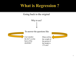
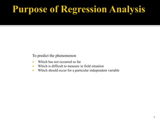
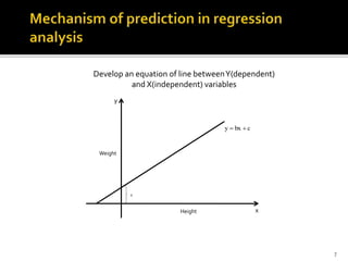
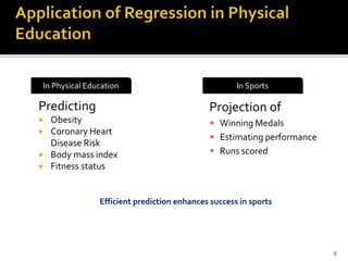
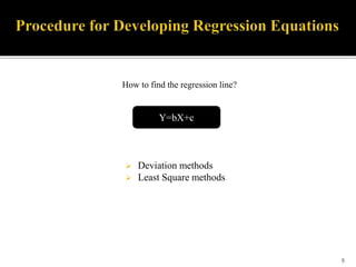
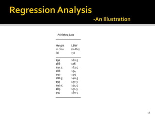
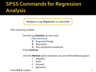
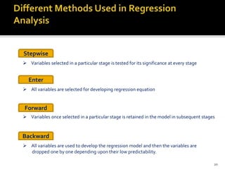
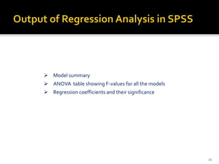
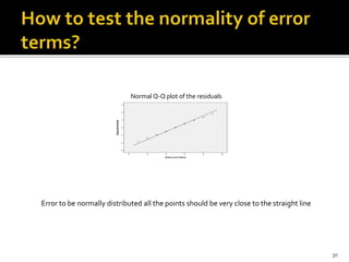
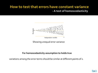
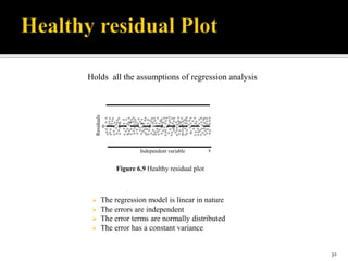
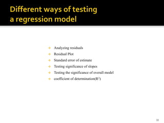
The document is a presentation by Dr. J.P. Verma that focuses on regression analysis as described in Chapter 9 of the book 'Sports Research with Analytical Solutions Using SPSS.' It covers the development of regression equations, methods for computing coefficients, and the implications of associations between independent and dependent variables in sports analytics. Specific examples of predicting body weight based on height using regression models are also discussed.

1. Presentation on Chapter 9
Presented by
Dr.J.P.Verma
MSc (Statistics), PhD, MA(Psychology), Masters(Computer Application)
Professor(Statistics)
Lakshmibai National Institute of Physical Education, Gwalior, India
(Deemed University)
Email: vermajprakash@gmail.com

2. To answer the questions like
Going back to the original
Why to use?
Can I predict
the fat % on the
basis of the
skinfolds?
What will be
the weight of
the person if
the height is
175 cms?
2

3.  Which has not occurred so far
 Which is difficult to measure in field situation
 Which should occur for a particular independent variable
To predict the phenomenon
3

4.  Simple Regression
 Multiple Regression
4

5. 5
This Presentation is based on
Chapter 9 of the book
Sports Research with Analytical
Solution Using SPSS
Published by Wiley, USA
Complete Presentation can be accessed on
Companion Website
of the Book
Request an Evaluation Copy For feedback write to vermajprakash@gmail.com

6. Developing Regression equation
With
One Dependent and one Independent variable
6

7. Develop an equation of line betweenY(dependent)
and X(independent) variables
y
x
cbxy 
c
Height
Weight
7

8. Predicting
 Obesity
 Coronary Heart
Disease Risk
 Body mass index
 Fitness status
Projection of
 Winning Medals
 Estimating performance
 Runs scored
In Physical Education In Sports
Efficient prediction enhances success in sports
8

9.  Deviation methods
 Least Square methods
How to find the regression line?
Y=bX+c
9

10. Regression equation ofY on X
)XX(rYY
x
y




YXrXrY
x
y
x
y







cbXY 
Regression equation of X onY
)YY(rXX
y
x 



b = regression coefficient
x
y
r


 c= slope YXr
x
y




…………(1)
…………(2)
Computing coefficients
10

11.  Yes if the slopes of the two equations are same
)xx(r)yy(
x
y




)xx(
r
)yy(
x
y




------(1)
------(2)
After solving )xx(r)yy(
x
y



 ------(3)
)yy(r)xx(
y
x 


 ------(4)
Equation (3) and (4) would be same if
x
y
x
y
r
r





 r2 = 1 or r = 1
Implication
If the relationship between two variables is either perfectly positive or perfectly negative one
can be estimated with the help of others with 100% accuracy, which is rarely the case.
11

12.  But association is a necessary prerequisite for inferring causation
 The independent variable must precede the dependent variable in time.
 The dependent and independent variables must be plausibly lined by a theory
 Regression focuses on association and not causation
12

13. Uses the concept of differential calculus
For n population points (x1,y1), (x2,y2), …….(xN , yN) an aggregate trend line can
be obtained
= β0 + β1xyˆ
where
: the estimated value of y
β0 : the population intercept (regression constant)
β1 : the population slope(regression coefficient)
yˆ
iyi = β0 + β1x +
For a particular score yi
Almost always Regression lines are developed on the basis of sample data hence
these β0 and β1 are estimated by the sample slope b0 and intercept b1
13

14. Infinite number of trend lines can be developed by changing
the slope b1 and intercept b0
yi = b0 + b1xi + i
For n sample data
the aggregate
regression line
= b0 + b1xyˆ
y
x
0b
xbbyˆ 10 
14

15. To find the best line so that the sum of squared
deviations is minimized
What the issue is?
For a particular point (x1,y1) in the scattergram
y
x
i
To get the best line needs to be minimized
   2
i10i
2
ii
2
i
2
)xbby()yˆy(S
- A least square method
iy
xbbyˆ 10 
0b
ii yˆy 
yˆyii 
or
y1 = b0 + b1x1 + 1
 2
i
2
S
15

16. Find the values of slope(b0) and intercept (b1) for which the S2 is minimized
This is done by using the differential
calculus
   2
10i
2
ii
2
)xbby()yˆy(S
0b
S


0)xbby(2
n
1i
i10i  

1b
S


 

n
1i
i10ii 0)xbby(x2
Solving we get normal
equations 

n
1i
i0
n
1i
i1 ynbxb


n
1i
ii
n
1i
i0
n
1i
2
i1 yxxbxb
 
   
 22
2
0
)x(xn
xyxxy
b
 221
xxn
yxxyn
b

  

xbbyˆ 10  - A line of best fit
16

17.  Data must be parametric
 There is no outliers in the data
 Variables are normally distributed(if not try log, square root, square, and
inverse transformation
 The regression model is linear in nature
 The errors are independent (no autocorrelation)
 The error terms are normally distributed
 There is no multicollinearity
 The error has a constant variance(assumption of homoscedasticity)
17

18. Athletes data
_________________
Height LBW
in cms (in lbs)
(x) (y)
_________________
191 162.5
186 136
191.5 163.5
188 154
190 149
188.5 140.5
193 157.3
190.5 154.5
189 151.5
192 160.5
_________________
18

19. After selecting variables
Click the tag Statistics on the screen
Check the box of
 R squared change
 Descriptive
 Part and partial correlations
Press Continue
Click the Method option and select any one of the following option
 Stepwise
 Enter
 Forward
 Backward
Press O.K for output
Analyze Regression Linear
19

20.  Variables selected in a particular stage is tested for its significance at every stage
Stepwise
 All variables are selected for developing regression equation
Enter
 Variables once selected in a particular stage is retained in the model in subsequent stages
Forward
 All variables are used to develop the regression model and then the variables are
dropped one by one depending upon their low predictability.
Backward
20

21.  Model summary
 ANOVA table showing F-values for all the models
 Regression coefficients and their significance
21

22. Model Summaryb
_________________________________________________
Model R R Square Adjusted R Std. Error of
Square the Estimate
1 .816 .666 .624 5.56
___________________________________________
a. Predictors: (Constant), Height
b. DependentVariable: BodyWeight
22

23. Regression analysis output for the Body weight example
______________________________________________________________________
Unstandardized Standardized
Coefficients Coefficients t Sig.
___________________________________
Model B Std. Error Beta
______________________________________________________________________
1 (Constant) - 517.047 167.719 -3.083 .015
Height 3.527 .883 .816 3.995(Click) .004
______________________________________________________________________
DependentVariable: Body weight R = 0.816 R2 = 0.666 Adjusted R2 =0.624
Look at the value of t computed in the last
slide and in the SPSS output
Y(Weight) = -517.047 + 3.527 ×(Height)
23

24. F = t2 = 3.9952 = 15.96
In simple regression significance of regression coefficient and model are same
Significance of the model is tested by F value in ANOVA
ANOVA table
___________________________________________________________________
Model Sum of Squares df Mean Square F Sig.
___________________________________________________________________
2 Regression 494.203 1 494.203 15.959 .004
Residual 247.738 8 30.967
Total 741.941 9
___________________________________________________________________
a. Predictors: (Constant), Height
Back to R2
24

25. Let’s See what the residual is?
25

26. Table Computation of residuals
____________________________________________
Height Body weight
in cms (in lbs)
x y
___________________________________________
191 162.5 156.61 5.89
186 136 138.975 -2.975
191.5 163.5 158.3735 5.1265
188 154 146.029 7.971
190 149 153.083 -4.083
188.5 140.5 147.7925 -7.2925
193 157.3 163.664 -6.364
190.5 154.5 154.8465 -0.3465
189 151.5 149.556 1.944
192 160.5 160.137 0.363
____________________________________________
yˆ
Residuals are estimates of experimental errors
For instance, for x= 188,
= -517.047 + 3.527×188 = 146.029yˆ
Maximum error: 7.97 1 lbs for height =188 cms
Minimum error: 0.3465 lbs for height = 190.5 cms.
Worst case
Best case
Useful in identifying the outliers
yˆy 
26

27. 184 186 188 190 192 194
Residuals
-10
-8
-6
-4
-2
0
2
4
6
8
Height in cms
Residual plot for the data on lean body mass and height
Obtained by plotting an ordered pair of (xi, y- )yˆ
Useful in testing the assumptions in the regression analysis
27

28. Independent variable x
0
Residuals
o
o
o
o
o
oo
o
o
o
o
o
oo
o
o
o
o
o
o
o
o
o
o
o
o o
o
oo
o
o o
o
o o
o
o
o
o
o
o
o
o
o
o
oo
o
oo
o
oo
o
o
oo
o
o
oo
oo
o
o
o
o
o
A curvilinear regression model
Residual plot
For low and high values of x the residuals are positives
And for middle value it is negative
28

29. o
o
oo
o
o
oo o
o
o
o
o
o
o
oo
o
o
o
o
o
o
oo o
o
o
o
o o
o
o
oo
o
o o
o
o o
o
o o
o
o
oo oo
o
oo
o o o o
o o
o
o
o
o
o
o o
o
o
x
0
Residuals
oo o
o oo
o
o o o
o
o
o o
o
o
oo
o o
o
o o
o
o
oo
o oo
o
ooo
o o
o
o
o
o
o oooo oo
o o
o o
o
o
o o
o
oo
Independent variable
Showing that the errors are related
No serial correlation should occur between a given error
term and itself over various time intervals
What is the pattern? : small positive residual occurs next to a small positive
residual and a larger positive residual occurs next to the large positive residual
29

30. Normal Q-Q plot of the residuals
Error to be normally distributed all the points should be very close to the straight line
30

31. Independent variable
o
o
o
o
o
oo
o
o
o
o
o
oo
o
o
o
o
o
o
o
o
o
o
o o
o
o
oo
o
o
o
o o
o
o
o
o
o
o
oo
o
o
o
o
o
o
oo
o
o
o
o
o
oo
o o
oo oo
o
o
o o
o
o o
o
oo o o
o
ooo
ooo
o
o
o
o
o o
o
o
oo
oo
o
o o
o
o o
oo o
o
o
oo oo
o o
o
o o o o
o o
o
o
o
o
o
o
o
o
o
o
o
o
oo
oo
o
o
o
x
0
Residuals
o oo o
o o
oo o
o o o
o o
o o o o o o o o
o
Showing unequal error variance
For homoscedasticity assumption to holds true
variations among the error terms should be similar at different points of x.
Back31

32.  The regression model is linear in nature
 The errors are independent
 The error terms are normally distributed
 The error has a constant variance
Holds all the assumptions of regression analysis
Independent variable
o
o
o
o
o
oo
o
o
o
o
o
oo
o
o
o o
o
o
o
o
o
o
o o
o
o
oo
o
o
o
o o
o
o
o
o
o
o
oo
o
o
o
o
o
oo
oo
o
o
o
o
o
o o
oo ooo o
o o
o
o
oo o o
o
ooo
ooo
o
o
o
oo o
o
o
oo
oo
o
o o
o
o o
o
o o
o
o
oo
oo
o o
oo o o o o o
o
o
o
o o
o
o
o
o
o
o
o
o oo
o
o
o
x
0
Residuals
o oo o
o o
oo o
o
o
oo o
o
o
o o
o
o o o
o o o o
o ooo
o o o oo o
o
o
o
o
oo
oo
oo oo o
o
o
o
o o
o o o
o o
o
o oo
o o o
o o
oo
ooo
o
o
o
o
o
o o
o
o
o
o
oo o
Figure 6.9 Healthy residual plot
32

33.  Analyzing residuals
 Residual Plot
 Standard error of estimate
 Testing significance of slopes
 Testing the significance of overall model
 coefficient of determination(R2)
33

34. 34
To buy the book
Sports Research With Analytical
Solutions Using SPSS
and all associated presentations click Here
Complete presentation is available on
companion website of the book
For feedback write to vermajprakash@gmail.comRequest an Evaluation Copy