Downloaded 30 times
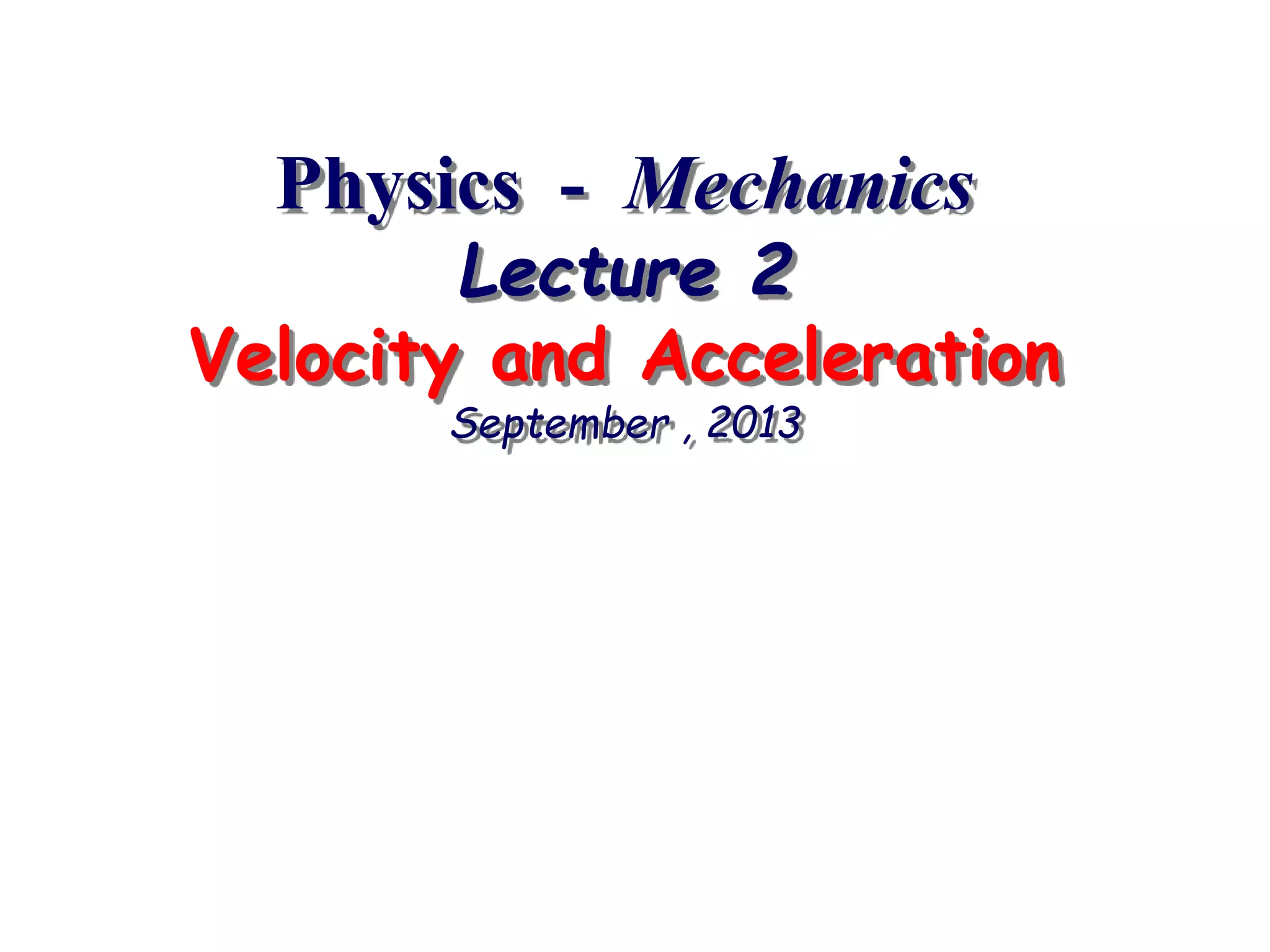

The document outlines a physics lecture series focusing on mechanics, specifically covering topics such as velocity, acceleration, and motion equations. It details the schedule of lectures, reading materials, and homework assignments from early January to mid-February 2012. Key concepts include graphical interpretation of velocity and acceleration, average and instantaneous values, and examples demonstrating these principles in real-world scenarios.
An overview of the lecture series on Mechanics focusing on Velocity and Acceleration, with mention of course details.
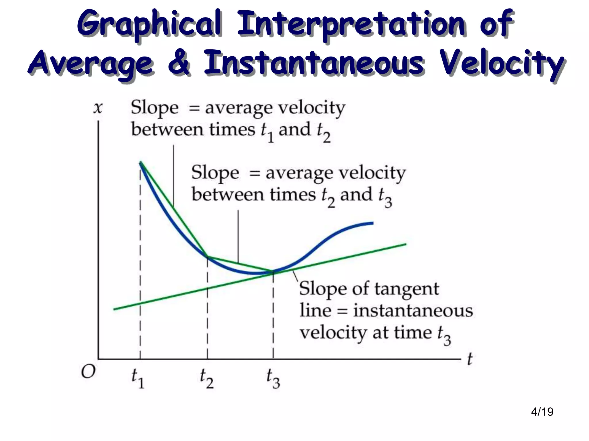
Introduction to velocity and acceleration, including graphical interpretations of average and instantaneous velocity.
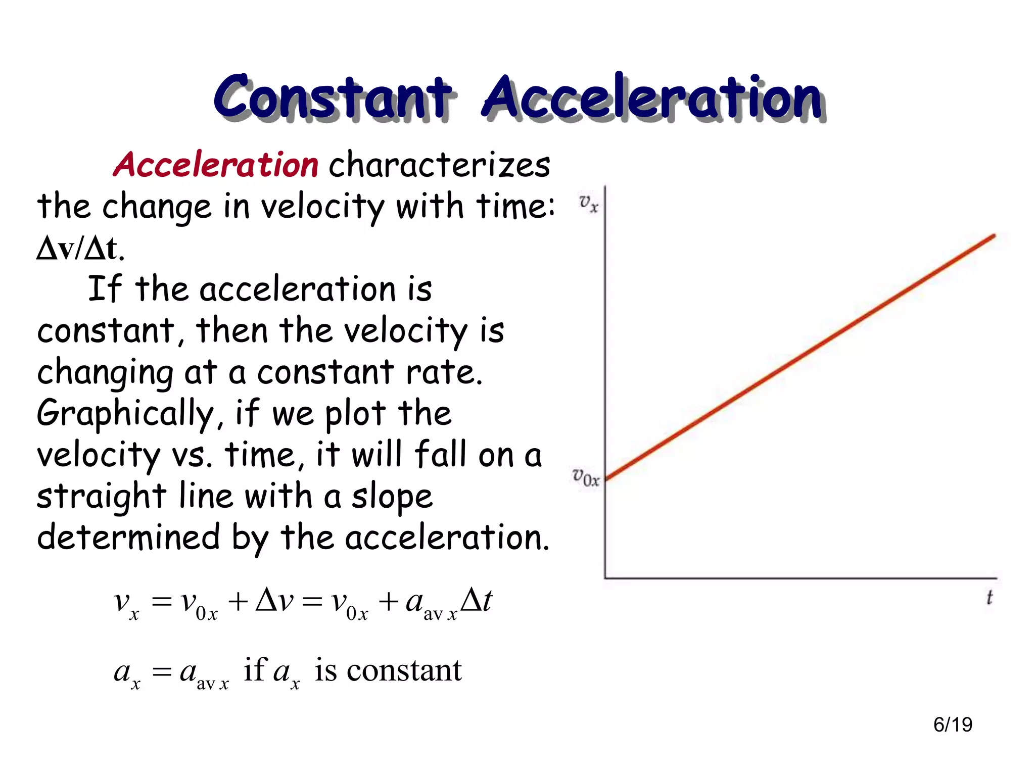
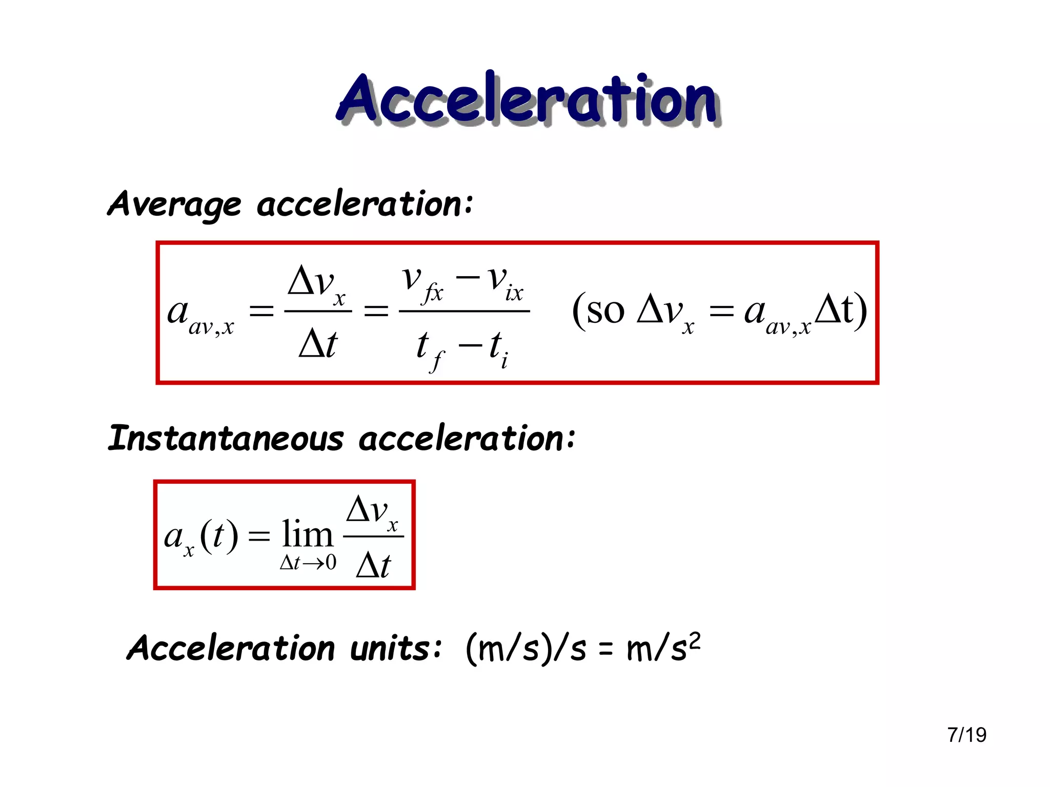
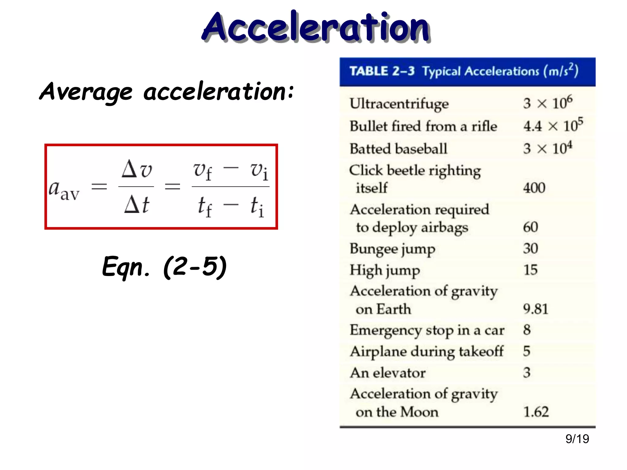
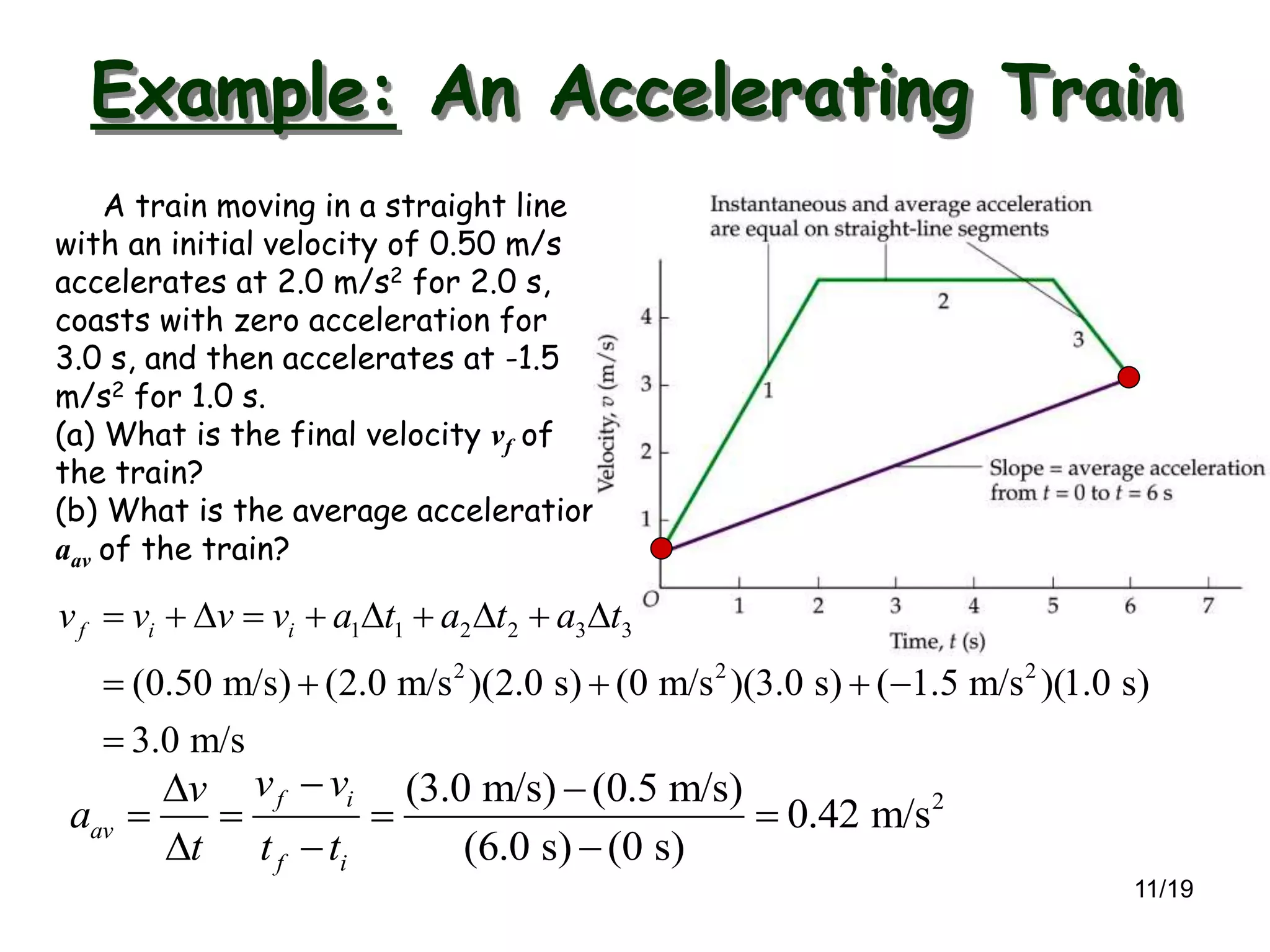
Detailed concepts of constant acceleration, average acceleration, and the relationship between velocity and acceleration.
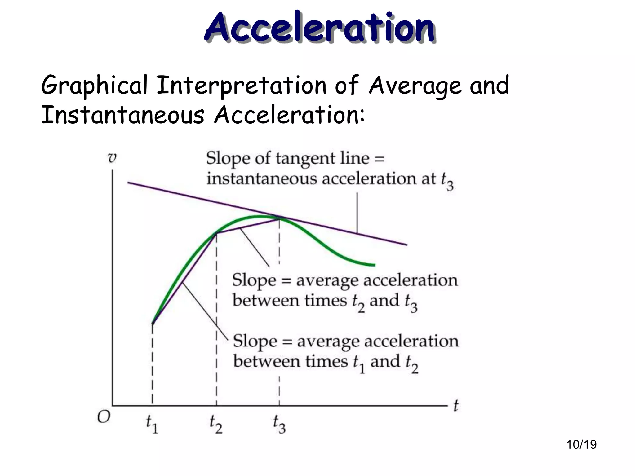
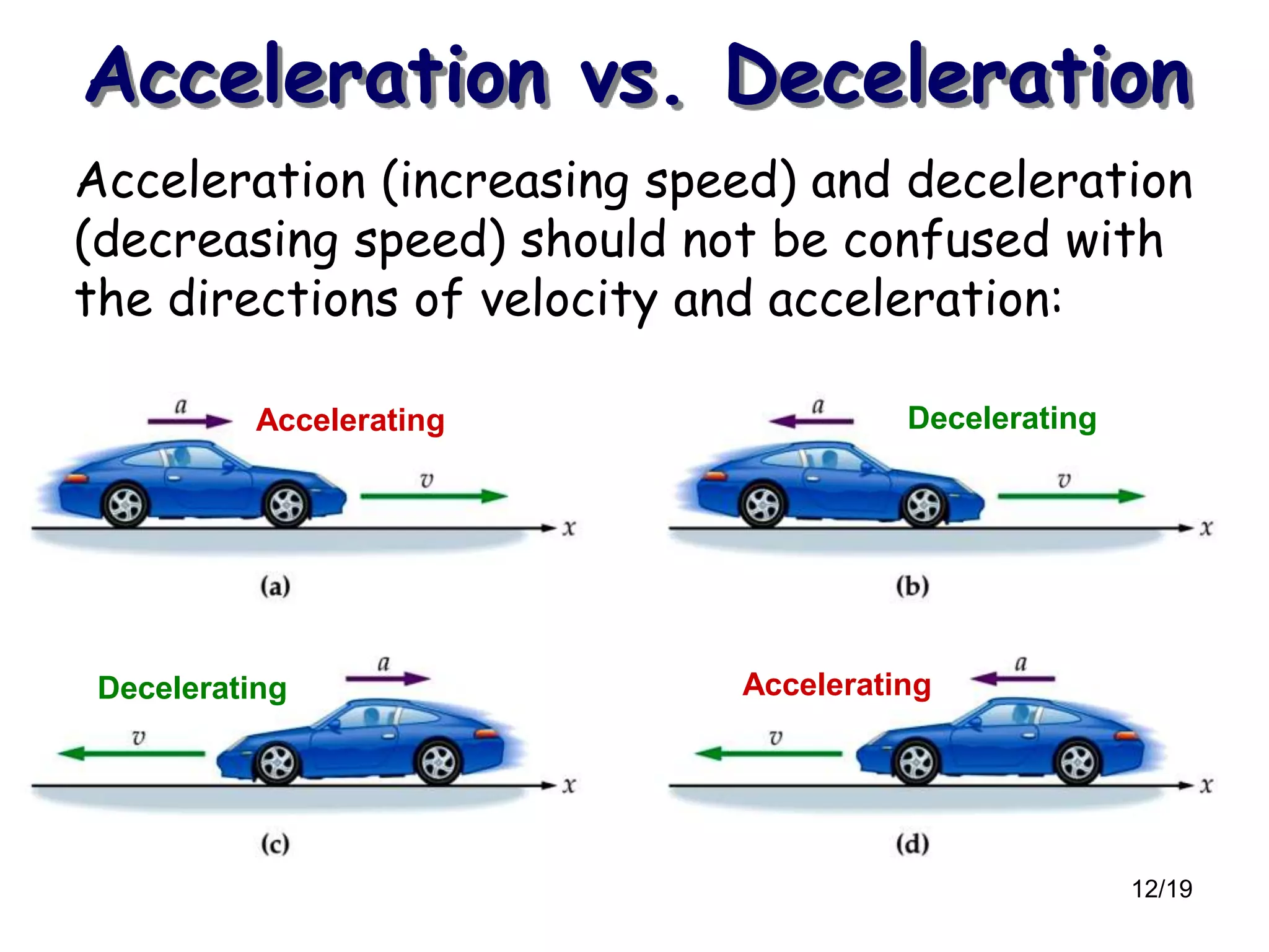
Graphical representations of average and instantaneous acceleration, distinguishing acceleration from deceleration.
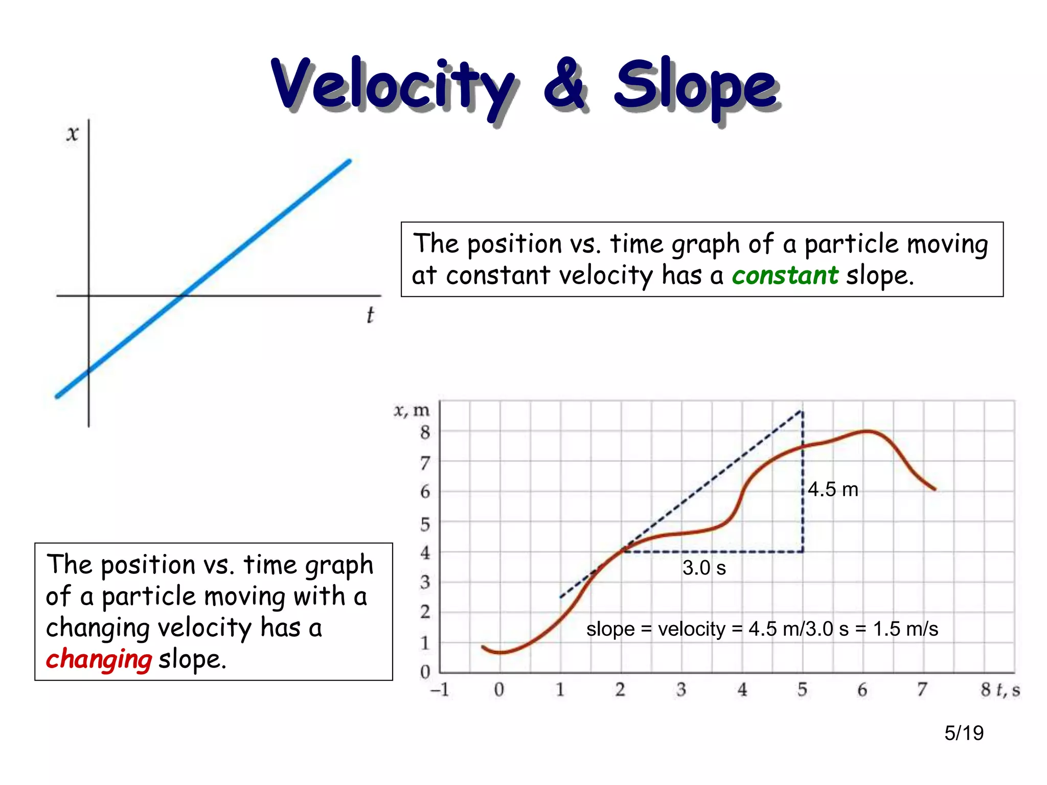
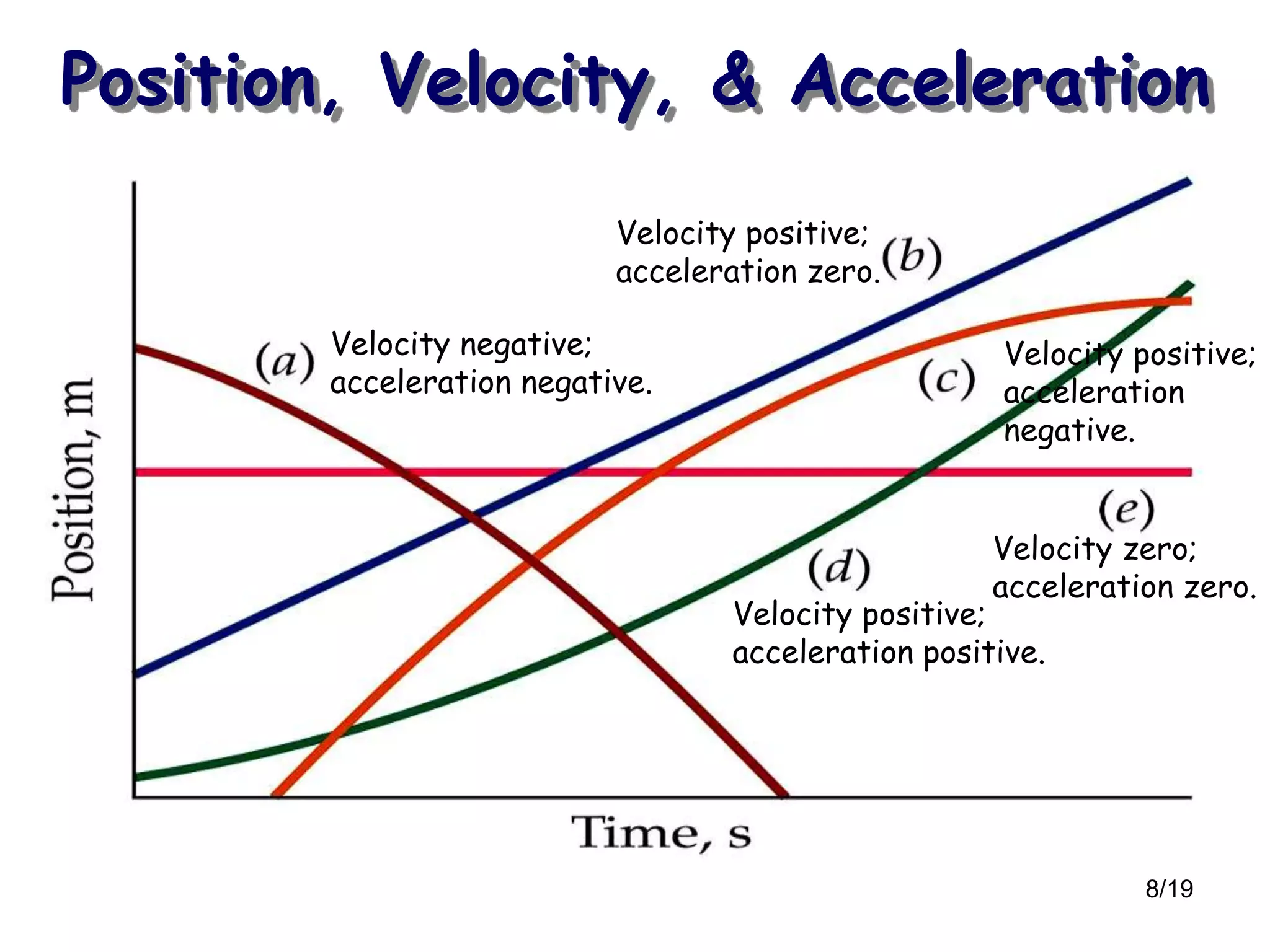
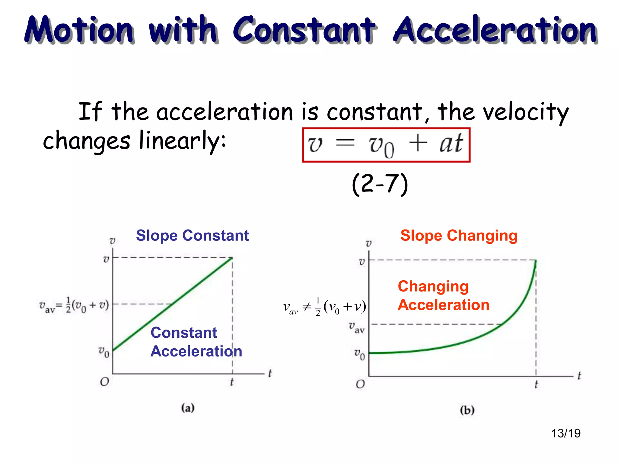
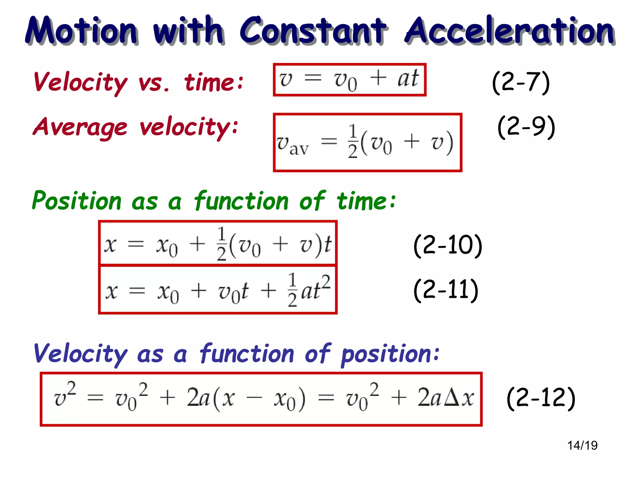
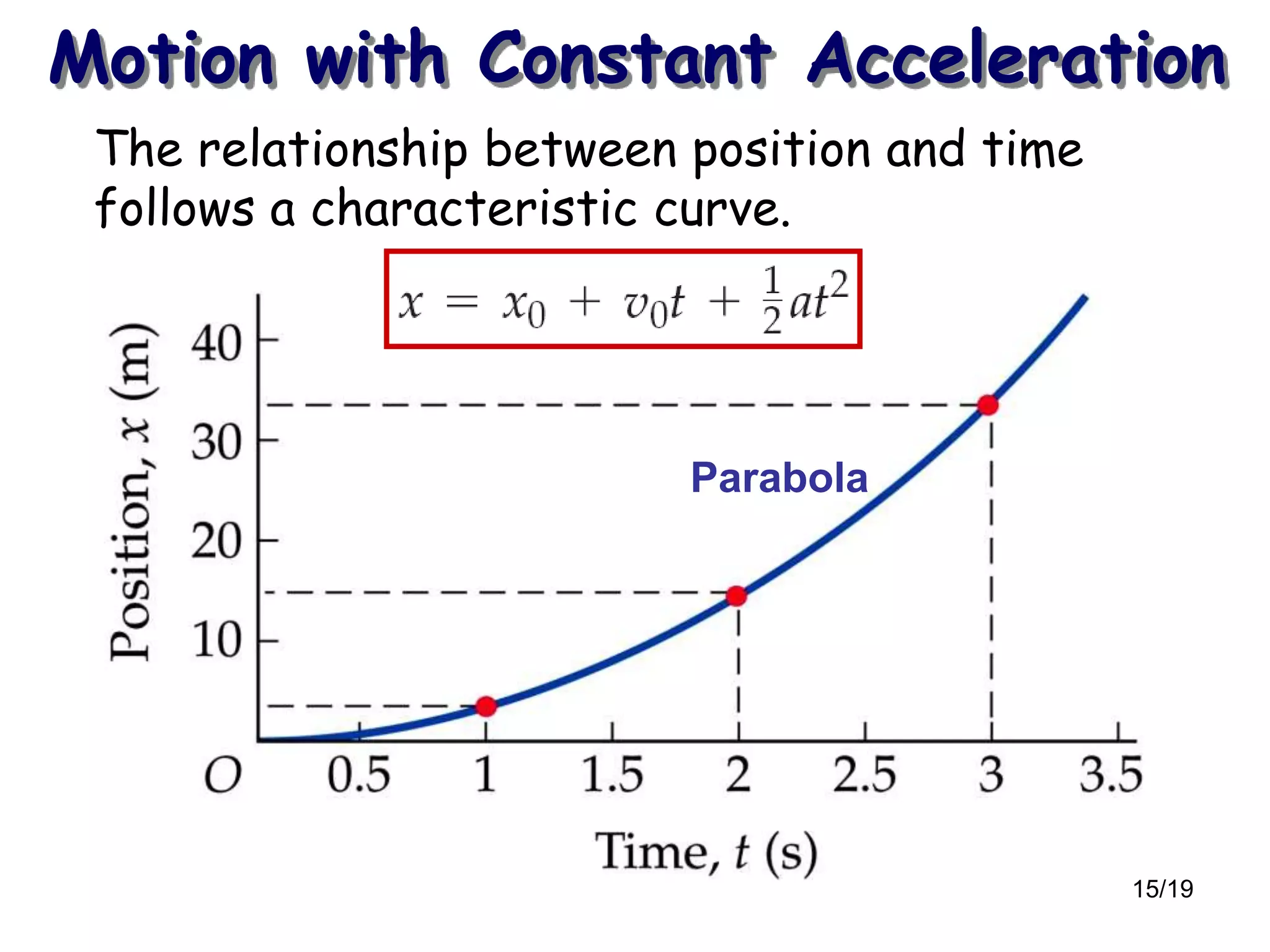
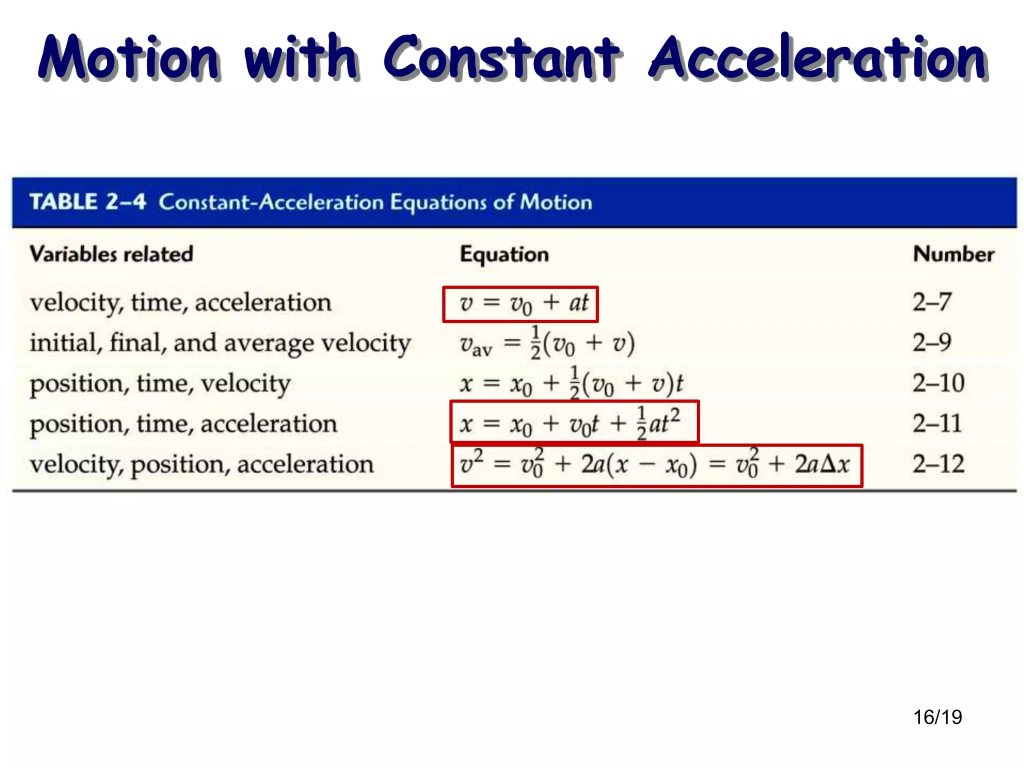
Analysis of motion with constant acceleration, illustrating linear changes in velocity and characteristics of position vs. time.
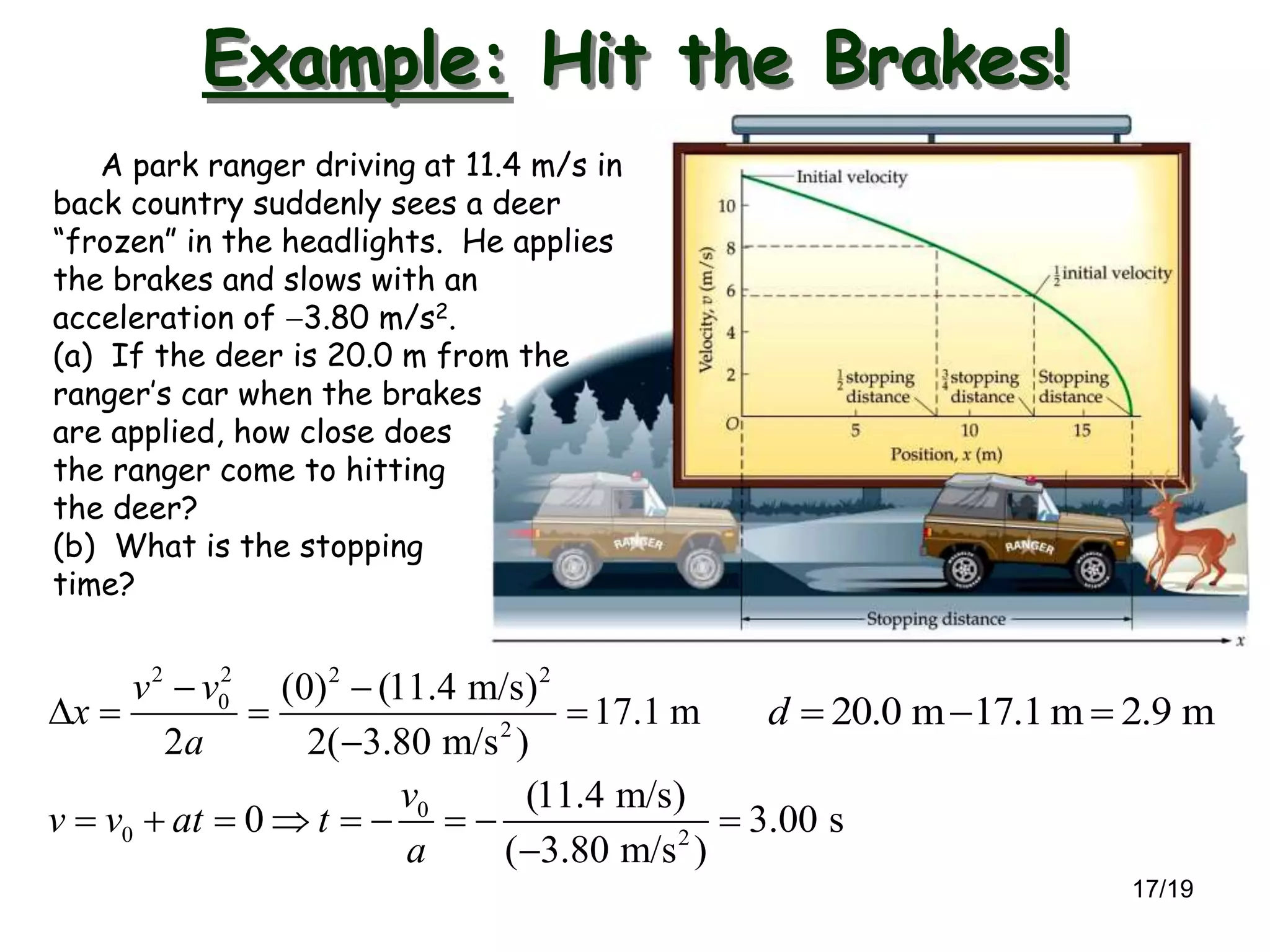
A real-world example involving a park ranger's braking scenario, focusing on calculations of distance and stopping time.