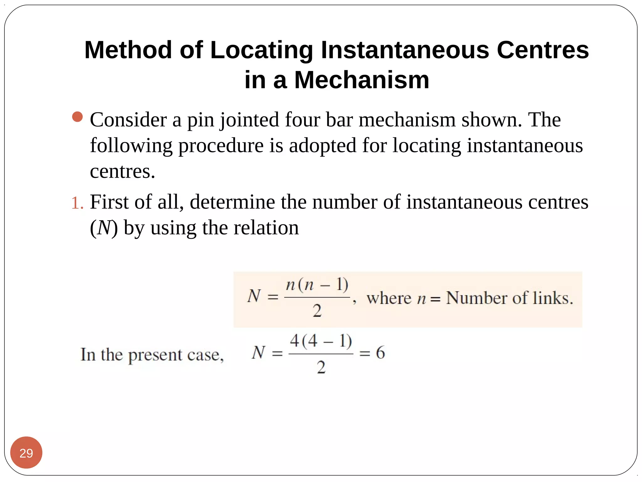
This document provides an overview of different methods for analyzing velocities and accelerations in linkages, including:
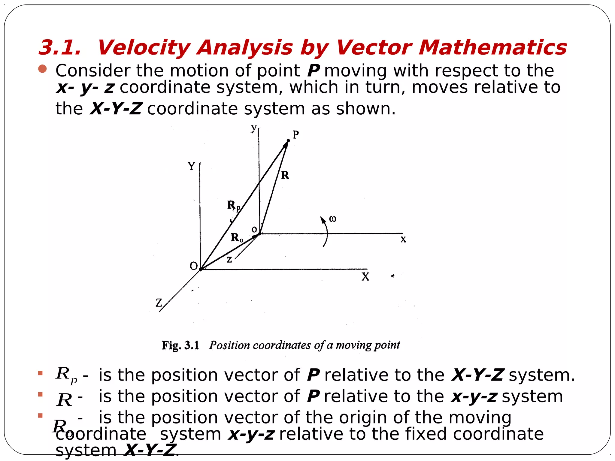
1) Vector mathematics, where velocities are expressed relative to fixed or moving coordinate systems.
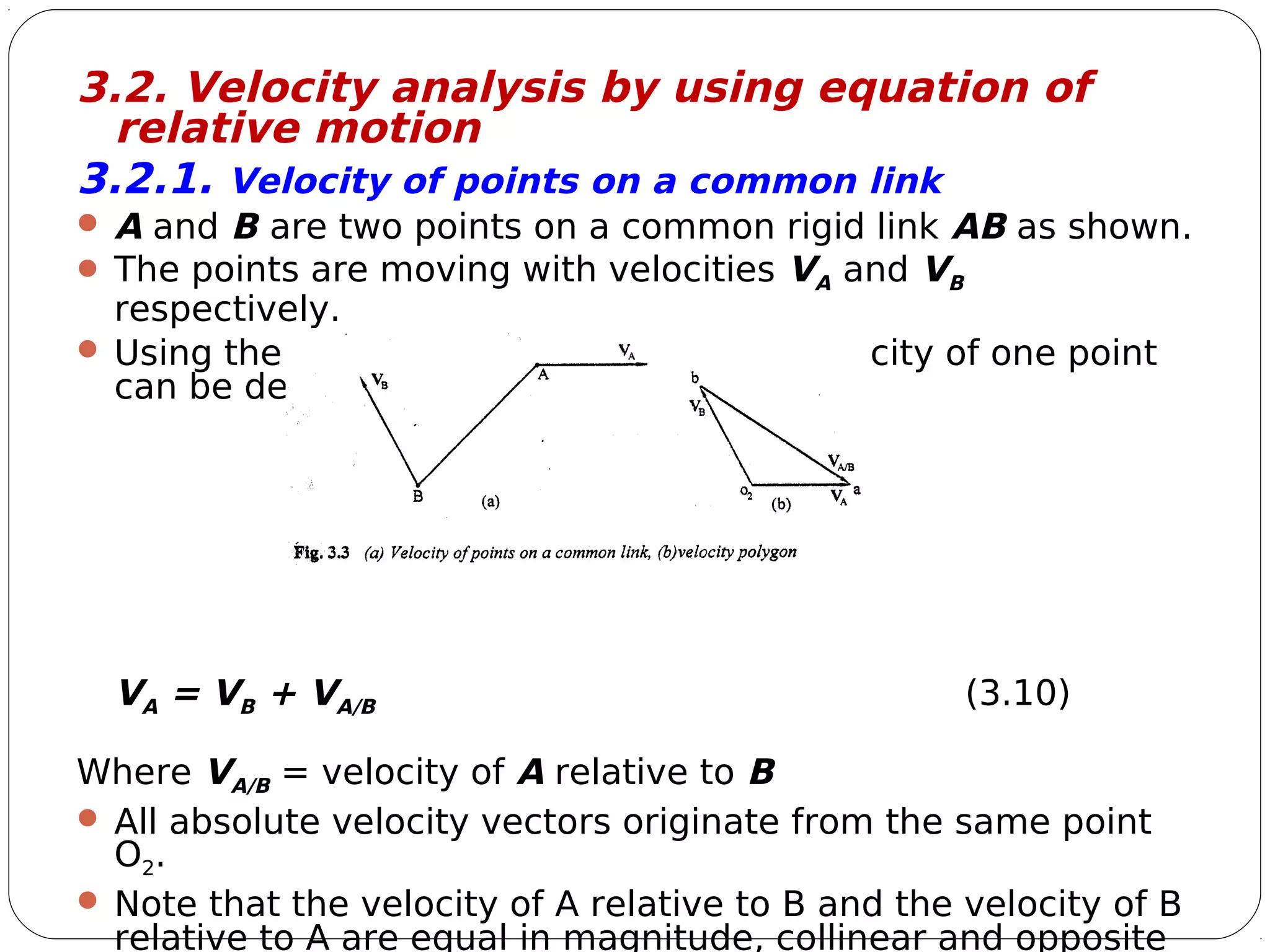
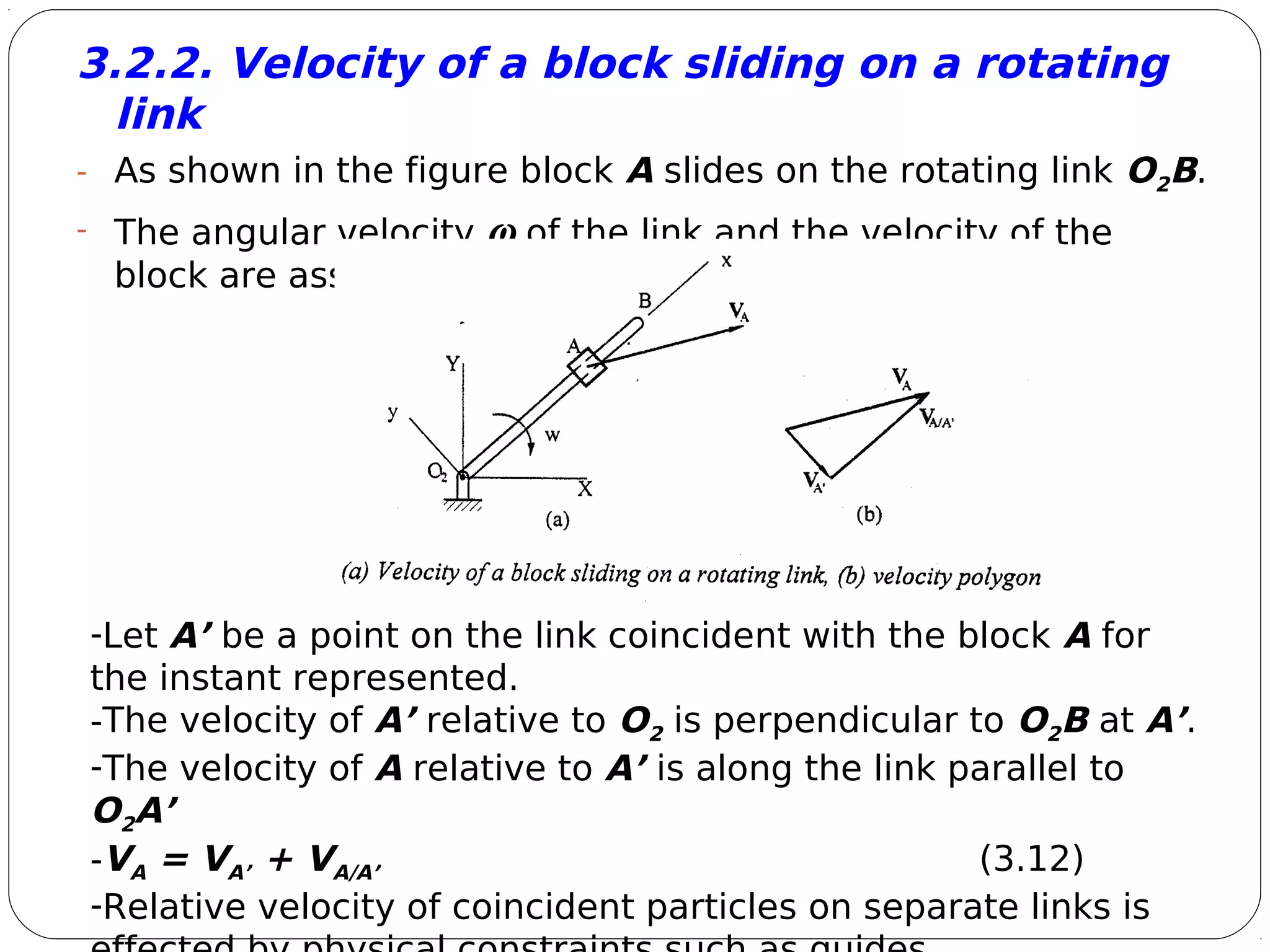
2) Equations of relative motion, which can be solved graphically or using trigonometric relations to determine velocities of points on moving links.
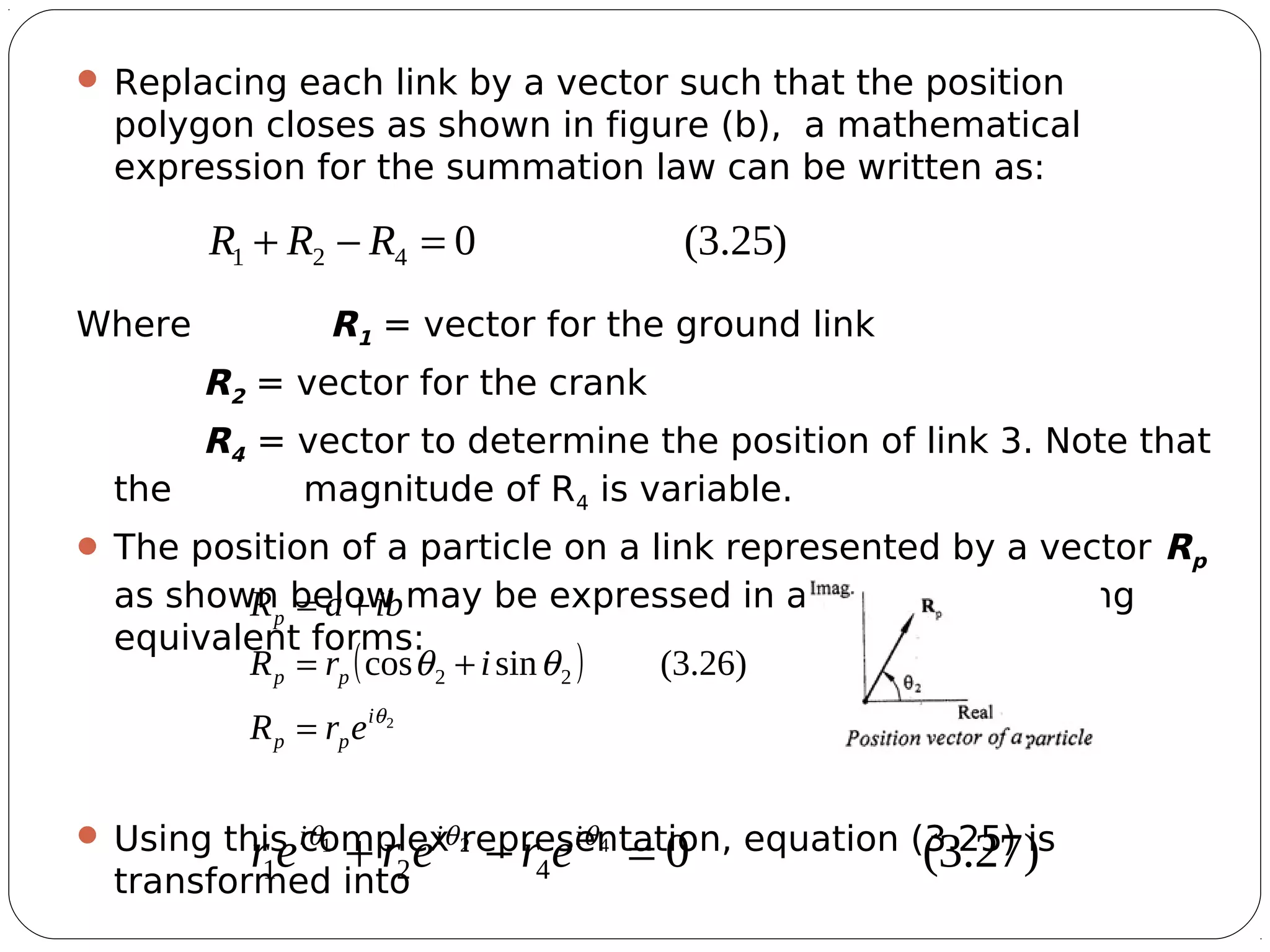
3) Complex numbers, where links are represented by vectors and the property that the sum of position vectors equals zero is used to determine velocities.
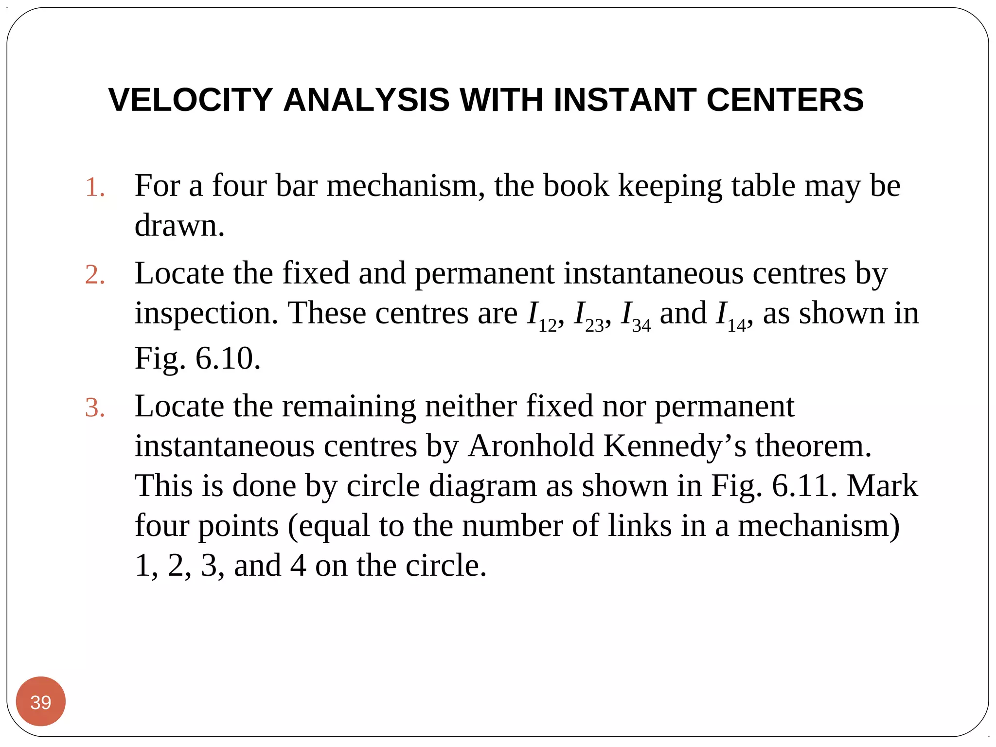
4) Instant center method, which identifies points where two moving bodies have the same velocity to analyze motion in a mechanism.
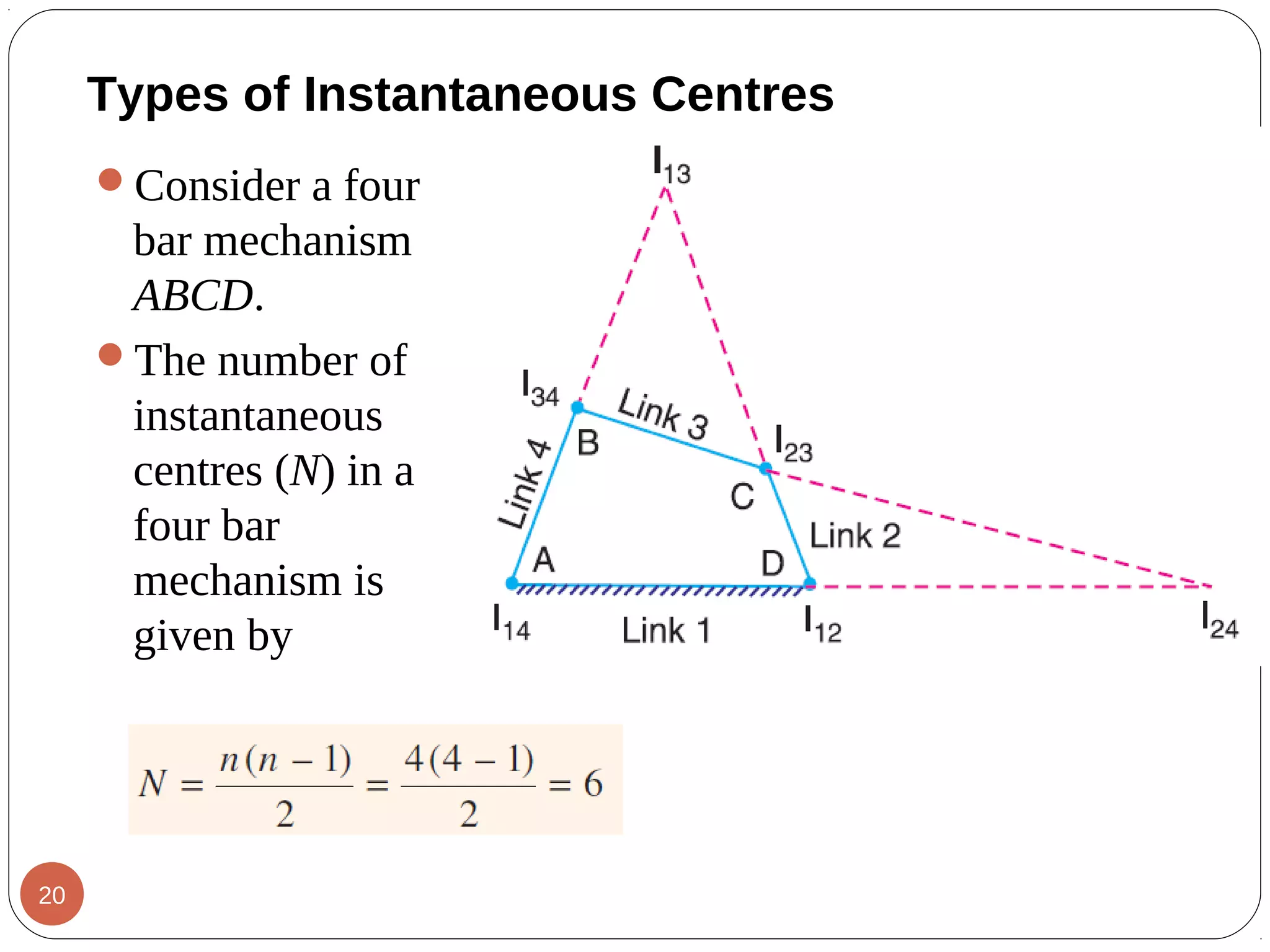
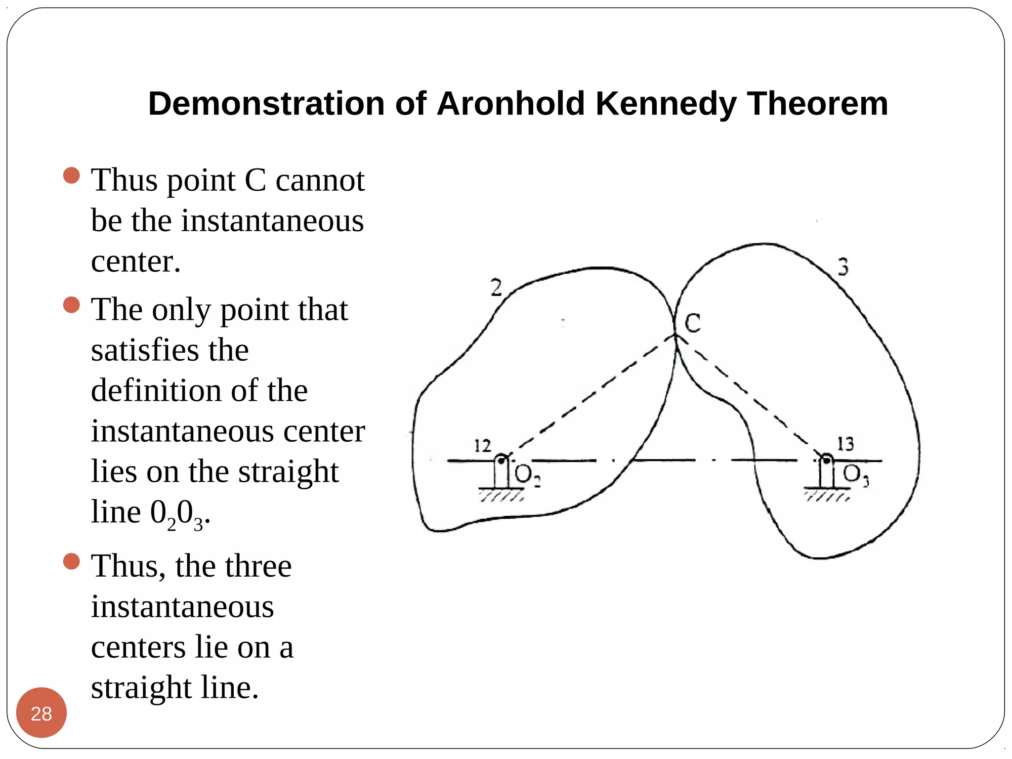
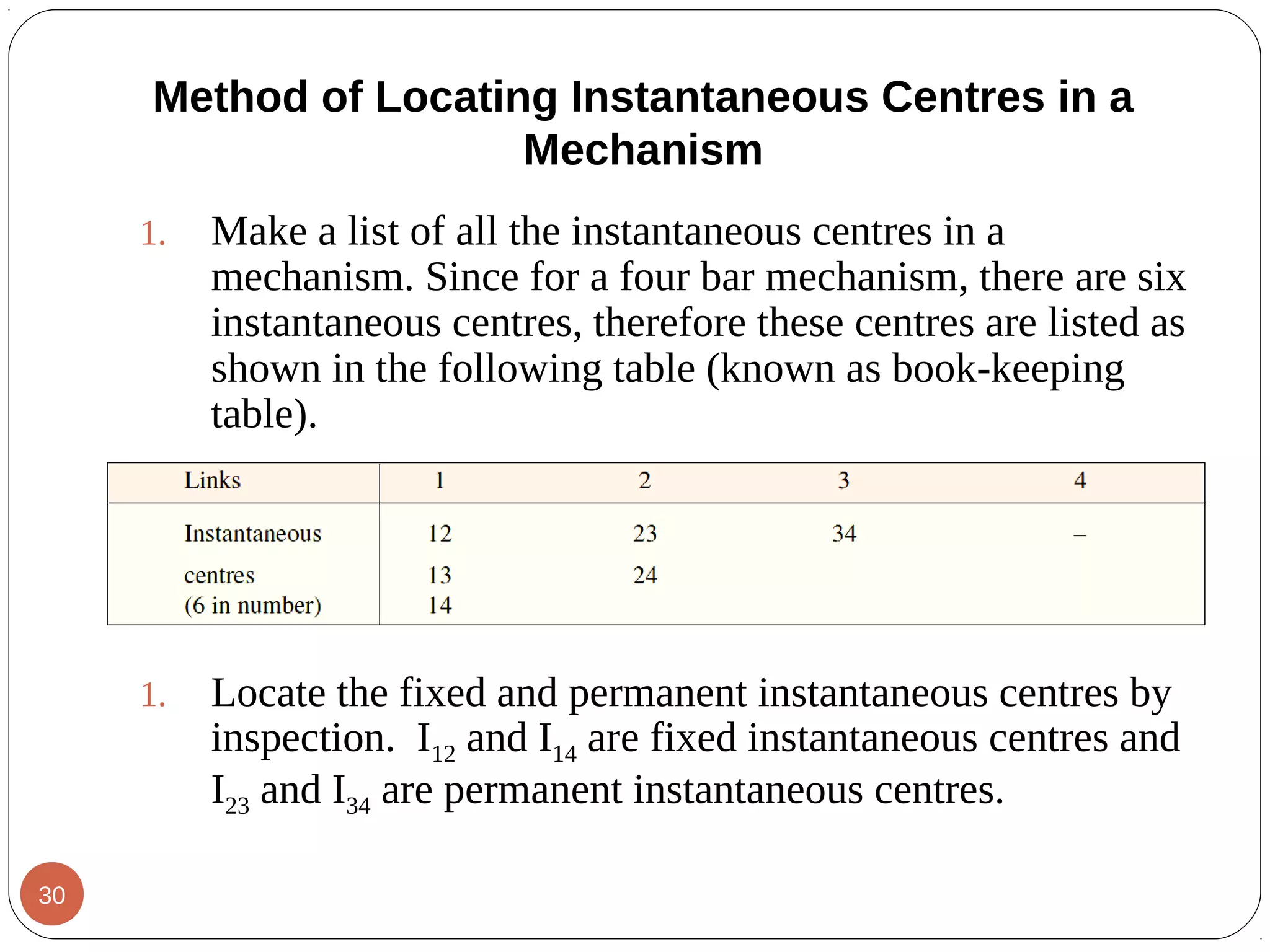
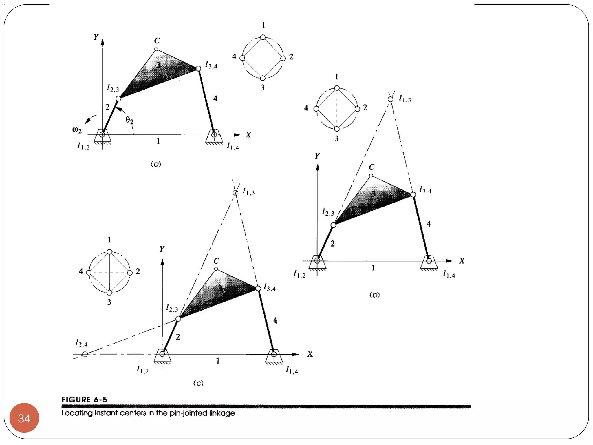
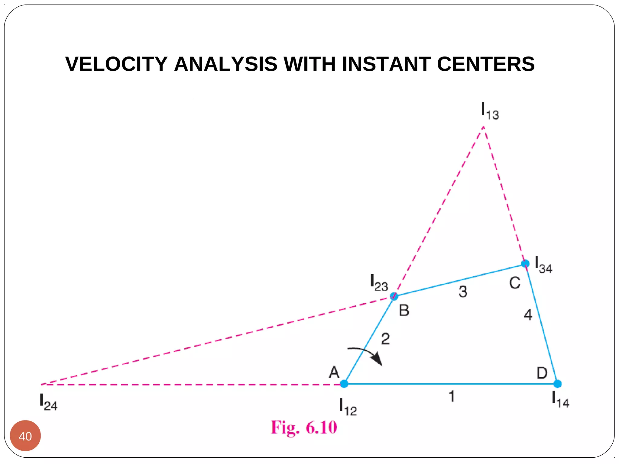
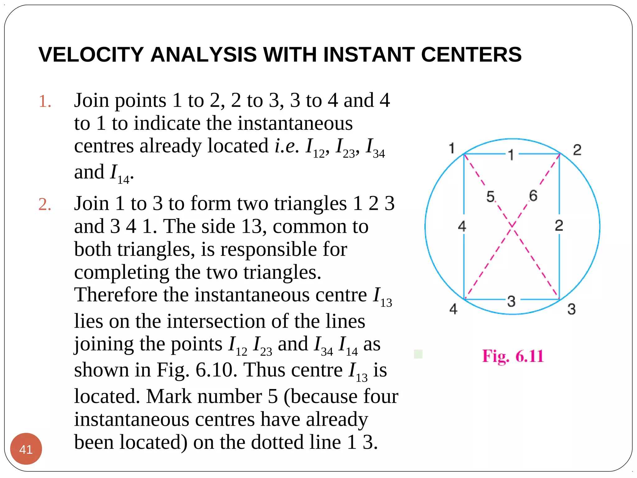
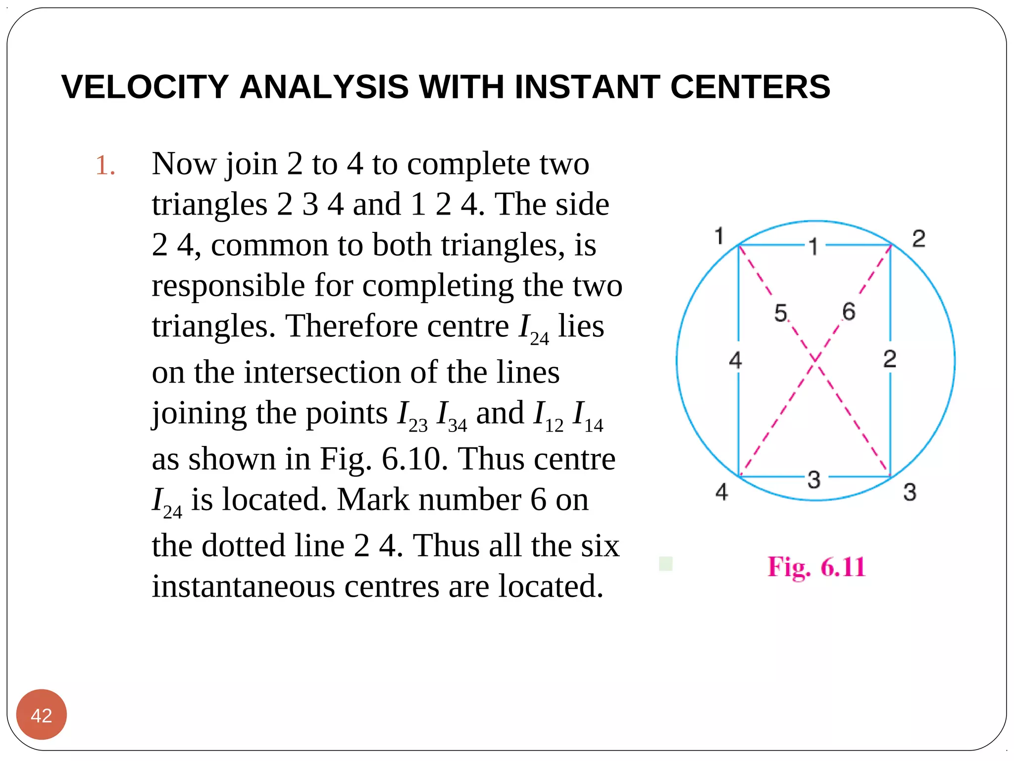
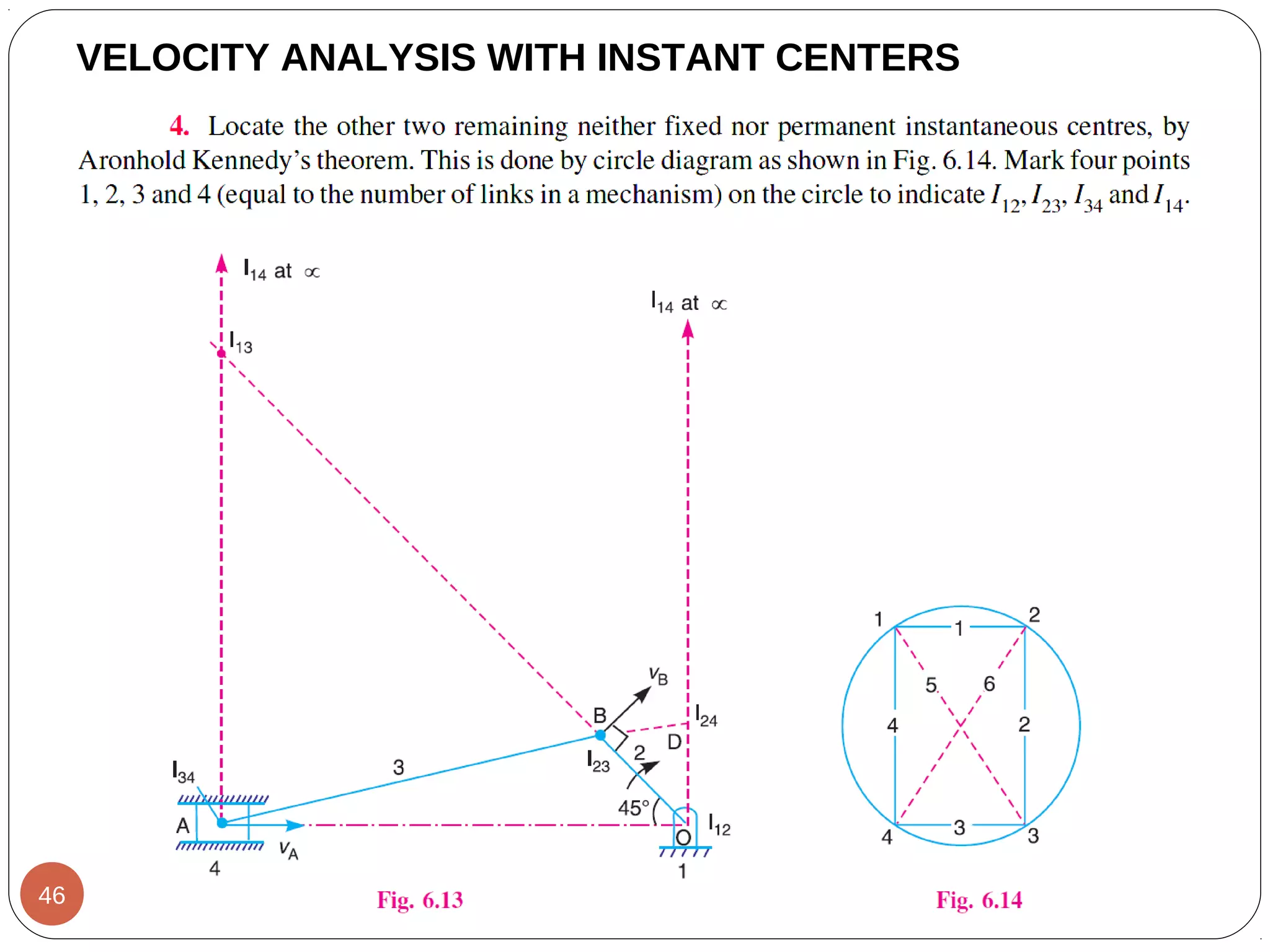
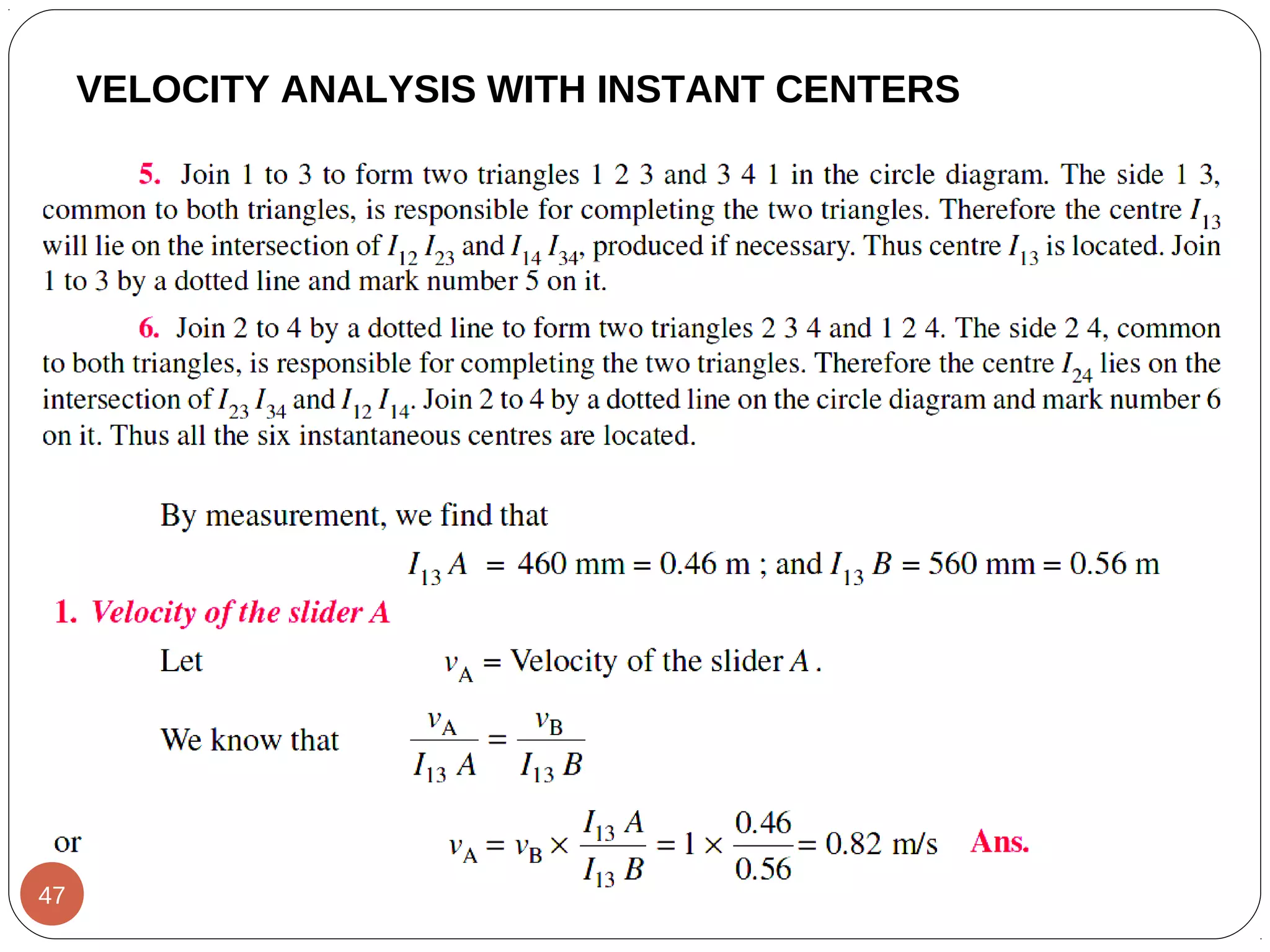
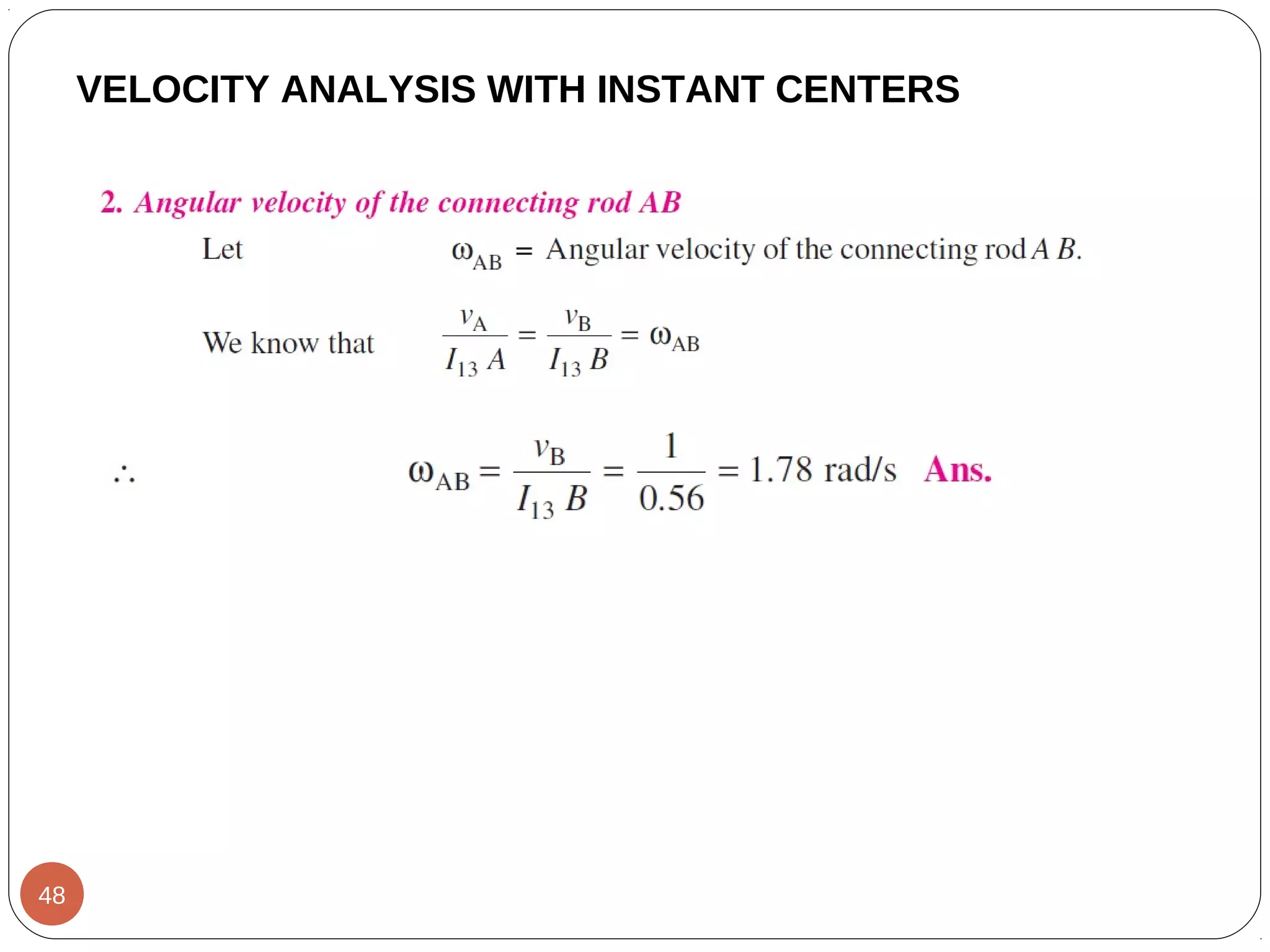
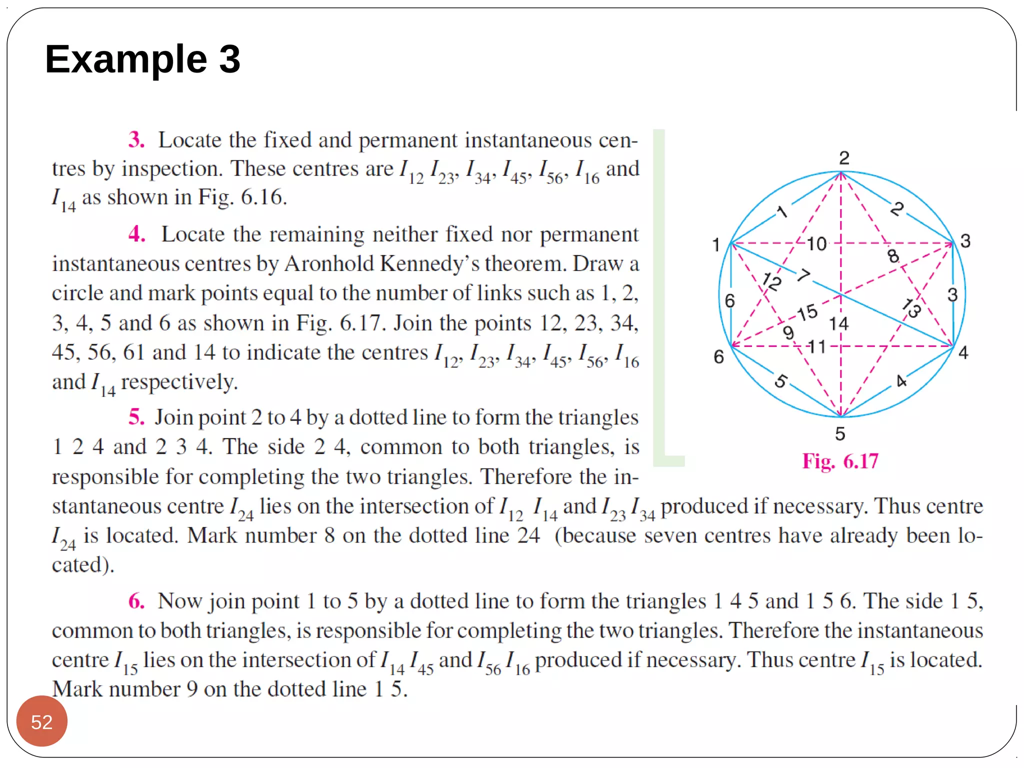
Unit 5- balancing of reciprocating masses, Dynamics of machines of VTU Syllabus prepared by Hareesha N Gowda, Asst. Prof, Dayananda Sagar College of Engg, Blore. Please write to hareeshang@gmail.com for suggestions and criticisms.
Unit-3 - Velocity and acceleration of mechanisms, Kinematics of machines of VTU Syllabus prepared by Hareesha N Gowda, Asst. Prof, Dayananda Sagar College of Engg, Blore. Please write to hareeshang@gmail.com for suggestions and criticisms.
Static force analysis, Unit-1 of Dynamics of machines of VTU Syllabus compiled by Hareesha N Gowda, Asst. Prof, Dayananda Sagar College of Engg, Blore. Please write to hareeshang@gmail.com for suggestions and criticisms.
the presentation consists of various important terms that are generally linked with the analysis of a common four bar mechanism which are as follows - coupler curves, toggle positions, transmission angles, mechanical advantage, acc analysis and coriolis component.
Unit 2- mechanisms, Kinematics of machines of VTU Syllabus prepared by Hareesha N Gowda, Asst. Prof, Dayananda Sagar College of Engg, Blore. Please write to hareeshang@gmail.com for suggestions and criticisms.
Kinematics Analysis of Parallel Mechanism Based on Force Feedback DeviceIJRES Journal
Kinematic analysis of mechanism is the fundamental work of force feedback device research.The
composition of Delta mechanism based on Omega.7 force feedback device was illustrated in this paper.The
kinematic loop equations of Delta mechanism was established according to its geometric relationship,also the
inverse kinematics solution of Delta mechanism were obtained. And the numerical forward kinematics were
calculated by Newton iteration algorithm.Finally,The analysis of velocity and acceleration was carried out
through matrix operations.Kinematic analysis of Delta mechanism provides a theoretical basis for following
study.
A two DOF spherical parallel platform posture analysis based on kinematic pri...IJRES Journal
Introducing the principle of kinematic analysis, the mathematical description and analysis
method of the constraints, pose and freedom were briefly outlined. A new 2-PSP & 1-S platform configuration
was presented. To derive attitude mathematical model of the platform, freedom and spinor system of the two
DOF spherical parallel platform were analyzed using kinematics principles. The results show, introducing the
concept of position and pose into the kinematic design, kinematic design method can be more widely used to
deal with the problem of the movement of the mechanism, so as to expand the application range of kinematic
design.
Linear quadratic regulator and pole placement for stabilizing a cart inverted...journalBEEI
The system of a cart inverted pendulum has many problems such as nonlinearity, complexity, unstable, and underactuated system. It makes this system be a benchmark for testing many control algorithm. This paper presents a comparison between 2 conventional control methods consist of a linear quadratic regulator (LQR) and pole placement. The comparison indicated by the most optimal steps and results in the system performance that obtained from each method for stabilizing a cart inverted pendulum system. A mathematical model of DC motor and mechanical transmission are included in a mathematical model to minimize the realtime implementation problem. From the simulation, the obtained system performance shows that each method has its advantages, and the desired pendulum angle and cart position reached.
International Journal of Engineering Inventions (IJEI) provides a multidisciplinary passage for researchers, managers, professionals, practitioners and students around the globe to publish high quality, peer-reviewed articles on all theoretical and empirical aspects of Engineering and Science.
The peer-reviewed International Journal of Engineering Inventions (IJEI) is started with a mission to encourage contribution to research in Science and Technology. Encourage and motivate researchers in challenging areas of Sciences and Technology.
Secure Communication and Implementation for a Chaotic Autonomous SystemNooria Sukmaningtyas
In this paper, a three-dimensional chaotic autonomous system is presented. The stability of the
equilibrium and the conditions of the Hopf bifurcation are studied by means of nonlinear dynamics theory.
Then, the circuit of chaotic system is structured out in Multisim platform by the unit circuit. The chaotic
system is applied to secure communications by linear feedback synchronization control. All simulations
results performed on three-dimensional chaotic autonomous system are verified the applicable of secure
communication.
Abstract— To be able to control a robot manipulator as.docxaryan532920
Abstract— To be able to control a robot manipulator as required
by its operation, it is important to consider the kinematic model in
design of the control algorithm. In robotics, the kinematic
descriptions of manipulators and their assigned tasks are utilized to
set up the fundamental equations for dynamics and control.. The
objective of this paper is to derive the complete forward kinematic
model (analytical and numerical) of a 6 DOF robotic arm (LR Mate
200iC from Fanuc Robotics) and validate it with the data provided by
robot’s software.
Keywords — forward kinematic, Denavit-Hartenberg parameters,
Robotic Toolbox
I. INTRODUCTION
Kinematics is the science of geometry in motion. It is
restricted to a pure geometrical description of motion by
means of position, orientation, and their time derivatives. In
robotics, the kinematic descriptions of manipulators and their
assigned tasks are utilized to set up the fundamental equations
for dynamics and control [1]. These non-linear equations are
used to map the joint parameters to the configuration of the
robot system. The Denavit and Hartenberg notation [2],[3]
gives us a standard methodology to write the kinematic
equations of a manipulator. This is especially useful for serial
manipulators where a matrix is used to represent the pose
(position and orientation) of one body with respect to another.
There are two important aspects in kinematic analysis of
robots: the Forward Kinematics problem and the Inverse
Kinematics problem. Forward kinematics refers to the use of
the kinematic equations of a robot to compute the position of
the end-effector from specified values for the joint parameters
Inverse kinematics refers to the use of the kinematics equations
of a robot to determine the joint parameters that provide a
desired position of the end-effector.
The purpose of this paper is to obtain the forward
kinematic analysis for the Fanuc LR Mate 200iC Robot, to
make model of robot using Robotic Toolbox® for MATLAB®
and validate it with the data provided by robot’s software. The
information can be use in the future design and production of
Daniel Constantin is with Military Technical Academy, Bucharest,
Romania; 39-49 George Cosbuc Blv., 050141, phone +40213354660; fax:
+40213355763; e-mail: [email protected]
Marin Lupoae is with Military Technical Academy, Bucharest, Romania;
e-mail: [email protected]
Cătălin Baciu is with Military Technical Academy, Bucharest, Romania;
e-mail: [email protected]
Dan-Ilie Buliga is with Military Technical Academy, Bucharest, Romania;
e-mail: [email protected]
the robot to make it faster and more accurate postwar period
for the defensive works executed in different countries around
the globe.
II. THEORETICAL ASPECTS
The forward kinematics problem is concerned with the
relationship between the individual joints of the robot
manipulator and the position and orientation of the tool or end-
effector.
A s ...
ANALYSIS AND SLIDING CONTROLLER DESIGN FOR HYBRID SYNCHRONIZATION OF HYPERCHA...IJCSEA Journal
Hybrid synchronization of chaotic systems is a research problem with a goal to synchronize the states of master and slave chaotic systems in a hybrid manner, namely, their even states are completely synchronized (CS) and odd states are anti-synchronized. This paper deals with the research problem of hybrid synchronization of chaotic systems. First, a detailed analysis is made on the qualitative properties of hyperchaotic Yujun system (2010). Then sliding controller has been derived for the hybrid synchronization of identical hyperchaotic Yujun systems, which is based on a general hybrid result derived in this paper.MATLAB simulations have been shown in detail to illustrate the new results derived for the hybrid synchronization of hyperchaotic Yujun systems. The results are proved using Lyapunov stability theory.
Similar to Chapter 3. velocity analysis (IC,GRAPHICAL AND RELATIVE VELOCITY METHOD) (20)
Industrial Training at Shahjalal Fertilizer Company Limited (SFCL)MdTanvirMahtab2
This presentation is about the working procedure of Shahjalal Fertilizer Company Limited (SFCL). A Govt. owned Company of Bangladesh Chemical Industries Corporation under Ministry of Industries.
Water scarcity is the lack of fresh water resources to meet the standard water demand. There are two type of water scarcity. One is physical. The other is economic water scarcity.
Automobile Management System Project Report.pdfKamal Acharya
The proposed project is developed to manage the automobile in the automobile dealer company. The main module in this project is login, automobile management, customer management, sales, complaints and reports. The first module is the login. The automobile showroom owner should login to the project for usage. The username and password are verified and if it is correct, next form opens. If the username and password are not correct, it shows the error message.
When a customer search for a automobile, if the automobile is available, they will be taken to a page that shows the details of the automobile including automobile name, automobile ID, quantity, price etc. “Automobile Management System” is useful for maintaining automobiles, customers effectively and hence helps for establishing good relation between customer and automobile organization. It contains various customized modules for effectively maintaining automobiles and stock information accurately and safely.
When the automobile is sold to the customer, stock will be reduced automatically. When a new purchase is made, stock will be increased automatically. While selecting automobiles for sale, the proposed software will automatically check for total number of available stock of that particular item, if the total stock of that particular item is less than 5, software will notify the user to purchase the particular item.
Also when the user tries to sale items which are not in stock, the system will prompt the user that the stock is not enough. Customers of this system can search for a automobile; can purchase a automobile easily by selecting fast. On the other hand the stock of automobiles can be maintained perfectly by the automobile shop manager overcoming the drawbacks of existing system.
Democratizing Fuzzing at Scale by Abhishek Aryaabh.arya
Presented at NUS: Fuzzing and Software Security Summer School 2024
This keynote talks about the democratization of fuzzing at scale, highlighting the collaboration between open source communities, academia, and industry to advance the field of fuzzing. It delves into the history of fuzzing, the development of scalable fuzzing platforms, and the empowerment of community-driven research. The talk will further discuss recent advancements leveraging AI/ML and offer insights into the future evolution of the fuzzing landscape.
Explore the innovative world of trenchless pipe repair with our comprehensive guide, "The Benefits and Techniques of Trenchless Pipe Repair." This document delves into the modern methods of repairing underground pipes without the need for extensive excavation, highlighting the numerous advantages and the latest techniques used in the industry.
Learn about the cost savings, reduced environmental impact, and minimal disruption associated with trenchless technology. Discover detailed explanations of popular techniques such as pipe bursting, cured-in-place pipe (CIPP) lining, and directional drilling. Understand how these methods can be applied to various types of infrastructure, from residential plumbing to large-scale municipal systems.
Ideal for homeowners, contractors, engineers, and anyone interested in modern plumbing solutions, this guide provides valuable insights into why trenchless pipe repair is becoming the preferred choice for pipe rehabilitation. Stay informed about the latest advancements and best practices in the field.
Courier management system project report.pdfKamal Acharya
It is now-a-days very important for the people to send or receive articles like imported furniture, electronic items, gifts, business goods and the like. People depend vastly on different transport systems which mostly use the manual way of receiving and delivering the articles. There is no way to track the articles till they are received and there is no way to let the customer know what happened in transit, once he booked some articles. In such a situation, we need a system which completely computerizes the cargo activities including time to time tracking of the articles sent. This need is fulfilled by Courier Management System software which is online software for the cargo management people that enables them to receive the goods from a source and send them to a required destination and track their status from time to time.
COLLEGE BUS MANAGEMENT SYSTEM PROJECT REPORT.pdfKamal Acharya
The College Bus Management system is completely developed by Visual Basic .NET Version. The application is connect with most secured database language MS SQL Server. The application is develop by using best combination of front-end and back-end languages. The application is totally design like flat user interface. This flat user interface is more attractive user interface in 2017. The application is gives more important to the system functionality. The application is to manage the student’s details, driver’s details, bus details, bus route details, bus fees details and more. The application has only one unit for admin. The admin can manage the entire application. The admin can login into the application by using username and password of the admin. The application is develop for big and small colleges. It is more user friendly for non-computer person. Even they can easily learn how to manage the application within hours. The application is more secure by the admin. The system will give an effective output for the VB.Net and SQL Server given as input to the system. The compiled java program given as input to the system, after scanning the program will generate different reports. The application generates the report for users. The admin can view and download the report of the data. The application deliver the excel format reports. Because, excel formatted reports is very easy to understand the income and expense of the college bus. This application is mainly develop for windows operating system users. In 2017, 73% of people enterprises are using windows operating system. So the application will easily install for all the windows operating system users. The application-developed size is very low. The application consumes very low space in disk. Therefore, the user can allocate very minimum local disk space for this application.
Welcome to WIPAC Monthly the magazine brought to you by the LinkedIn Group Water Industry Process Automation & Control.
In this month's edition, along with this month's industry news to celebrate the 13 years since the group was created we have articles including
A case study of the used of Advanced Process Control at the Wastewater Treatment works at Lleida in Spain
A look back on an article on smart wastewater networks in order to see how the industry has measured up in the interim around the adoption of Digital Transformation in the Water Industry.
Sachpazis:Terzaghi Bearing Capacity Estimation in simple terms with Calculati...Dr.Costas Sachpazis
Terzaghi's soil bearing capacity theory, developed by Karl Terzaghi, is a fundamental principle in geotechnical engineering used to determine the bearing capacity of shallow foundations. This theory provides a method to calculate the ultimate bearing capacity of soil, which is the maximum load per unit area that the soil can support without undergoing shear failure. The Calculation HTML Code included.
Sachpazis:Terzaghi Bearing Capacity Estimation in simple terms with Calculati...
Chapter 3. velocity analysis (IC,GRAPHICAL AND RELATIVE VELOCITY METHOD)
1. 1
Velocity Analysis of Linkages
Chapter 3
Mechanisms of Machinery
(MEng 3301)
Mechanical Engineering
Department
Prepared by: Addisu D. November, 2013
2. 2
Velocity Analysis of Linkages
Velocities and accelerations in mechanisms are determined
by different methods.
i. Velocity and acceleration analysis using vector mathematics
velocity and acceleration of a point are expressed
relative to fixed or moving coordinates.
i. Velocity and acceleration analysis using equations of
relative motion
Can be solved graphically by velocity and acceleration
polygons or by using trigonometric relations.
i. Velocity and acceleration analysis by using complex
numbers.
ii. Vectors velocity analysis using the instant center method.
3. 3
3.1. Velocity Analysis by Vector Mathematics
Consider the motion of point P moving with respect to the
x- y- z coordinate system, which in turn, moves relative to
the X-Y-Z coordinate system as shown.
- is the position vector of P relative to the X-Y-Z system.
- is the position vector of P relative to the x-y-z system
- is the position vector of the origin of the moving
coordinate system x-y-z relative to the fixed coordinate
system X-Y-Z.
pR
R
oR
4. 4
The position vector of P relative to the X-Y-Z system Rp is
expressed as:
(3.1)
Introducing unit vectors i, j, and k along the x, y, and z axes
respectively,
= xi + yj + zk (3.2)
Velocity of P relative to the X-Y-Z coordinate system is
(3.3)
- is the velocity of the origin of x-y-z system
relative to the fixed system
(3.4)
RRRV opp
+==
oo VR
=
( )
)()( kzjyixkzjyix
zkyjxi
dt
d
R
+++++=
++=
RRR op
+=
R
5. 5
Let
(3.5)
note that
(3.6)
Where ω is the angular velocity vector of x-y-z system relative
to X-Y-Z.
⇒
(3.7)
- Thus the velocity of P relative to the moving coordinate system
is
(3.8)
Vkzjyix =++
kk
jj
ii
×=
×=
×=
ω
ω
ω
R
zkyjxi
kzjyixkzjyix
×=
++×=
×+×+×=++
ω
ω
ωωω
)(
)()()(
RVR
×+= ω
6. 6
∴ the velocity of point P relative to the fixed system is:
= velocity of the origin of the x-y-z system relative to
the X-Y- Z system
= velocity of point p relative to x-y-z system
ω = angular velocity of the x-y-z system relative to X-Y-Z
system
= position vector of P with respect to the origin of the
x-y-z system
)9.3(RVVV op
×++= ω
oV
V
R
7. 7
3.2. Velocity analysis by using equation of
relative motion
3.2.1. Velocity of points on a common link
A and B are two points on a common rigid link AB as shown.
The points are moving with velocities VA and VB
respectively.
Using the equation of relative motion, velocity of one point
can be determined relative to the other.
VA = VB + VA/B (3.10)
Where VA/B = velocity of A relative to B
All absolute velocity vectors originate from the same point
O2.
Note that the velocity of A relative to B and the velocity of B
relative to A are equal in magnitude, collinear and opposite
8. 8
3.2.2. Velocity of a block sliding on a rotating
link
- As shown in the figure block A slides on the rotating link O2B.
- The angular velocity ω of the link and the velocity of the
block are assumed to be known.
-Let A’ be a point on the link coincident with the block A for
the instant represented.
-The velocity of A’ relative to O2 is perpendicular to O2B at A’.
-The velocity of A relative to A’ is along the link parallel to
O2A’
-VA = VA’ + VA/A’ (3.12)
-Relative velocity of coincident particles on separate links is
9. 9
3.2.3 . Relative velocity of crank and
connecting rod
Let ω2 be the angular velocity of the crank O2A.
Velocity of B can be determined using the velocity of point
A as the reference which can easily be determined.
VB = VA + VB/A
(3.16)
Where
VA is known both in magnitude and direction;
VB is known in direction, magnitude is unknown;
10. 10
3.3. Velocity Analysis by Complex
Numbers
Most of the systems of analysis using complex polar
notation are based on the following fundamental law:
If the elements of a mechanism are replaced by position
vectors such that their sum is zero, then their time
derivatives are also equal to zero.
This law means that if one takes any linkage or mechanism
and replaces the members of the mechanism by vectors
such that their sum is zero, then the sum of the velocity
vectors is zero, so also the sum of the acceleration vectors.
Considering the slider crank shown:
Link 2 is the driver (crank) and has
a constant angular velocity ω2 & for
the instant under consideration an
angular position of θ2.
Dimensions of linkages are assumed
to be known, so the angular position
of the follower, link 4, can be obtained.
11. 11
Replacing each link by a vector such that the position
polygon closes as shown in figure (b), a mathematical
expression for the summation law can be written as:
Where R1 = vector for the ground link
R2 = vector for the crank
R4 = vector to determine the position of link 3. Note that
the magnitude of R4 is variable.
The position of a particle on a link represented by a vector Rp
as shown below may be expressed in any of the following
equivalent forms:
Using this complex representation, equation (3.25) is
transformed into
)25.3(0421 =−+ RRR
( )
2
)26.3(sincos 22
θ
θθ
i
pp
pp
p
erR
irR
ibaR
=
+=
+=
)27.3(0421
421 =−+ θθθ iii
ererer
12. 12
Differentiating the above equation we obtain
Note that r1 and θ1 are constants and r4 is variable.
Let
Separating equation (3.29) into real and imaginary terms:
The unknown quantities in the above pair of equations are ω4
and
solving for these unknown variables:
)28.3(0442
44422 =−− θθθ
θθ iii
ereireir
ii ωθ =
)29.3(0442
44422 =−− θθθ
ωω iii
ereireir
)30.3(0sincossin
0cossincos
44444222
44444222
=+−−
=−−
θωθθω
θωθθω
rrr
rrr
4r
)31.3()cos(
)sin(
24
4
22
4
24224
θθ
ω
ω
θθω
−=
−=
r
r
rr
13. Definition
The definition of an instant center of a velocity is a point,
common to two bodies in plane motion, which the point has the
same instantaneous velocity in each body.
The instantaneous center of velocity is defined as the
instantaneous location of a pair of coincident points of two
different rigid bodies for which the absolute velocities of the
two points are equal.
It may also be defined as the location of a pair of coincident
points of two different rigid bodies for which the apparent
velocity of one of the points is zero as seen by an observer on
the other body.
3.4. Analysis of Velocity Vectors by
Instant-Center Method.
13
14. Velocity Analysis by Instant-center Method
The instantaneous center method of analyzing the motion in
a mechanism is based upon the concept that any
displacement of a body (or a rigid link) having motion in
one plane, can be considered as a pure rotational motion of a
rigid link as a whole about some centre, known as
instantaneous centre or virtual centre of rotation.
Consider two points A and B on a rigid link. Let vA and vB be
the velocities of points A and B, whose directions are given
by angles α and β as shown in Fig. If vA is known in
magnitude and direction and vB in direction only, then the
magnitude of vB may be determined by the instantaneous
centre method as discussed below :
14
15. Velocity Analysis by Instant-center Method
Draw AI and BI perpendiculars
to the directions vA and vB
respectively.
Let these lines intersect at I,
which is known as
instantaneous centre or virtual
centre of the link.
The complete rigid link is to
rotate or turn about the centre I.
Since A and B are the points on
a rigid link, therefore there
cannot be any relative motion
between them along the line
AB.
15
17. Properties of the Instantaneous Centre
The following properties of the instantaneous centre are
important from the subject point of view :
A rigid link rotates instantaneously relative to another link at
the instantaneous centre for the configuration of the
mechanism considered.
The two rigid links have no linear velocity relative to each
other at the instantaneous centre. At this point (i.e.
instantaneous centre), the two rigid links have the same linear
velocity relative to the third rigid link.
In other words, the velocity of the instantaneous centre relative
to any third rigid link will be same whether the instantaneous
centre is regarded as a point on the first rigid link or on the
second rigid link.
17
18. Number of Instantaneous Centres in a
Mechanism
The number of instantaneous centers in a constrained
kinematic chain is equal to the number of possible
combinations of two links. The number of pairs of links or
the number of instantaneous centers is the number of
combinations of n links taken two at a time.
Mathematically, number of instantaneous centers,
18
19. Types of Instantaneous Centres
The instantaneous centers for a mechanism are of the
following three types :
Fixed instantaneous centers,
Permanent instantaneous centres, and
Neither fixed nor permanent instantaneous centres.
The first two types i.e. fixed and permanent instantaneous
centres are together known as primary instantaneous
centres and the third type is known as secondary
instantaneous centres.
19
20. Consider a four
bar mechanism
ABCD.
The number of
instantaneous
centres (N) in a
four bar
mechanism is
given by
Types of Instantaneous Centres
20
21. The instantaneous centres I12 and I14 are called the fixed
instantaneous centres as they remain in the same place for
all configurations of the mechanism.
The instantaneous centres I23 and I34 are the permanent
instantaneous centres as they move when the mechanism
moves, but the joints are of permanent nature.
The instantaneous centres I13 and I24 are neither fixed nor
permanent instantaneous centres as they vary with the
configuration of the mechanism.
Types of Instantaneous Centres
21
22. Location of Instantaneous Centres
The following rules may be used in locating the
instantaneous centres in a mechanism :
1. When the two links are connected by a pin joint (or pivot
joint), the instantaneous centre lies on the centre of the pin.
Such a instantaneous centre is of permanent nature, but if one
of the links is fixed, the instantaneous centre will be of fixed
type.
22
23. 1. When the two links have a pure rolling contact (i.e. link 2
rolls without slipping upon the fixed link 1 which may be
straight or curved), the instantaneous centre lies on their
point of contact. The velocity of any point A on the link 2
relative to fixed link 1 will be perpendicular to I12 A and is
proportional to I12 A . In other words
Location of Instantaneous Centres
23
24. 1. When the two links have a sliding contact, the
instantaneous centre lies on the common normal at the
point of contact. We shall consider the following three
cases :
When the link 2 (slider) moves on fixed link 1 having straight
surface, the instantaneous centre lies at infinity and each point
on the slider have the same velocity.
When the link 2 (slider) moves on fixed link 1 having curved
surface, the instantaneous centre lies on the centre of curvature
of the curvilinear path in the configuration at that instant.
When the link 2 (slider) moves on fixed link 1 having constant
radius of curvature, the instantaneous centre lies at the centre of
curvature i.e. the centre of the circle, for all configuration of
the links.
Location of Instantaneous Centres
24
26. Aronhold Kennedy (or Three Centres in
Line) Theorem
The Arnhold- Kennedy
theorem states that:
When three bodies move
relative to one another
they have three
instantaneous centers, all
of which lie on the same
straight line.
For the four-bar linkage
shown in Fig., centers 12,
23, 34 and 14 are located
by inspection.
26
27. The intersection of the perpendiculars to the velocities of
points A and B yield the instantaneous center 13 which is
the point about which link 3 appears to rotate relative to
link 1 or vice versa.
Demonstration:
Consider the three bodies shown below. Link 1 is the stationary link
and links 2 and 3 rotate about the centers 12 and 13.
Let us assume that the instantaneous center 23 lies at point C. Then
the velocity of C as a point on link 2 is Vc2 and as a point on link 3
is Vc3 both perpendicular to 02C and 03C, respectively.
The directions of the velocities obviously do not coincide, hence,
the velocity of C as a point on link 2 is different from the velocity
of point C as a point on link 3.
Aronhold Kennedy (or Three Centres in Line)
Theorem
27
28. Thus point C cannot
be the instantaneous
center.
The only point that
satisfies the
definition of the
instantaneous center
lies on the straight
line 0203.
Thus, the three
instantaneous
centers lie on a
straight line.
Demonstration of Aronhold Kennedy Theorem
28
29. Method of Locating Instantaneous Centres
in a Mechanism
Consider a pin jointed four bar mechanism shown. The
following procedure is adopted for locating instantaneous
centres.
1. First of all, determine the number of instantaneous centres
(N) by using the relation
29
30. 1. Make a list of all the instantaneous centres in a
mechanism. Since for a four bar mechanism, there are six
instantaneous centres, therefore these centres are listed as
shown in the following table (known as book-keeping
table).
1. Locate the fixed and permanent instantaneous centres by
inspection. I12 and I14 are fixed instantaneous centres and
I23 and I34 are permanent instantaneous centres.
Method of Locating Instantaneous Centres in a
Mechanism
30
31. 1. Locate the remaining neither fixed nor permanent instantaneous
centres (or secondary centres) by Kennedy’s theorem. This is done
by circle diagram as shown in Fig. 6.8 (b). Mark points on a circle
equal to the number of links in a mechanism. In the present case,
mark 1, 2, 3, and 4 on the circle.
Method of Locating Instantaneous Centres in a
Mechanism
31
32. 1. Join the points by solid lines to show that these centres are already
found. In the circle diagram [Fig. 6.8 (b)] these lines are 12, 23, 34
and 14 to indicate the centres I12, I23, I34 and I14.
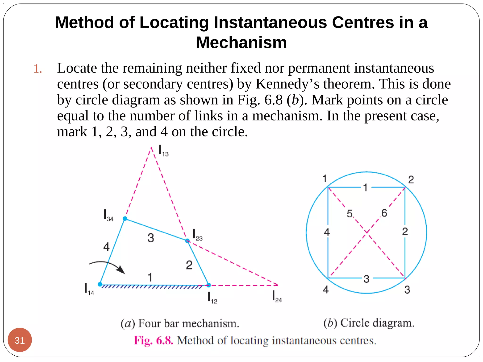
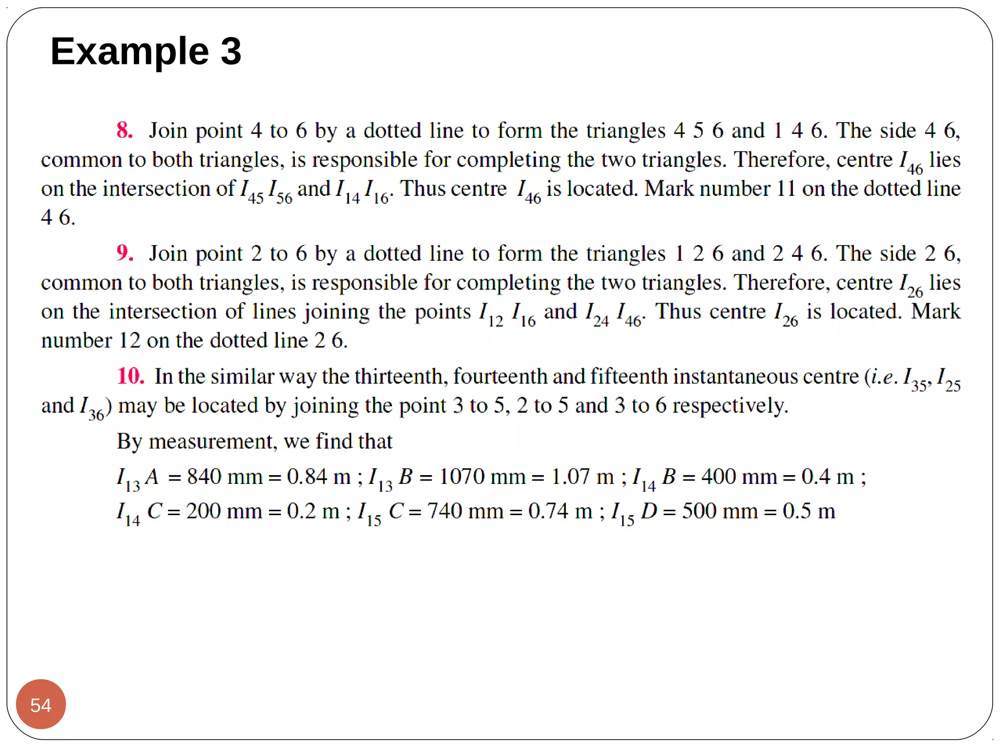
2. In order to find the other two instantaneous centres, join two such
points that the line joining them forms two adjacent triangles in the
circle diagram. The line which is responsible for completing two
triangles, should be a common side to the two triangles. In Fig. 6.8
(b), join 1 and 3 to form the triangles 123 and 341 and the
instantaneous centre* I13 will lie on the intersection of I12 I23 and I14
I34, produced if necessary, on the mechanism. Thus the
instantaneous centre I 13 is located. Join 1 and 3 by a dotted line on
the circle diagram and mark number 5 on it. Similarly the
instantaneous centre I24 will lie on the intersection of I12 I14 and I23
I34, produced if necessary, on the mechanism. Thus I24 is located.
Join 2 and 4 by a dotted line on the circle diagram and mark 6 on it.
Hence all the six instantaneous centres are located.
Method of Locating Instantaneous Centres in a
Mechanism
32
36. VELOCITY ANALYSIS WITH INSTANT
CENTERS
Once the ICs have been found, they can be used to do a
very rapid graphical velocity analysis of the linkage.
From the definition of the instant center, both links sharing
the instant center will have identical velocity at that point.
36
37. Example 1. In a pin
jointed four bar
mechanism shown, AB =
300 mm, BC = CD = 360
mm, and AD = 600 mm.
The angle BAD = 60°.
The crank AB rotates
uniformly at 100 r.p.m.
Locate all the
instantaneous centres and
find the angular velocity
of the link BC.
VELOCITY ANALYSIS WITH INSTANT CENTERS
37
38. Example 1
Solution. Given : NAB = 100 r.p.m
or ωAB = 2 × 100/60 = 10.47 rad/s
Since the length of crank AB = 300 mm = 0.3 m, therefore
velocity of point B on link AB,
vB = ωAB × AB = 10.47 × 0.3 = 3.141 m/s
Location of instantaneous centres
The instantaneous centres are located as discussed below:
Since the mechanism consists of four links (i.e. n = 4 ),
therefore number of instantaneous centres,
38
39. 1. For a four bar mechanism, the book keeping table may be
drawn.
2. Locate the fixed and permanent instantaneous centres by
inspection. These centres are I12, I23, I34 and I14, as shown in
Fig. 6.10.
3. Locate the remaining neither fixed nor permanent
instantaneous centres by Aronhold Kennedy’s theorem.
This is done by circle diagram as shown in Fig. 6.11. Mark
four points (equal to the number of links in a mechanism)
1, 2, 3, and 4 on the circle.
VELOCITY ANALYSIS WITH INSTANT CENTERS
39
41. VELOCITY ANALYSIS WITH INSTANT CENTERS
1. Join points 1 to 2, 2 to 3, 3 to 4 and 4
to 1 to indicate the instantaneous
centres already located i.e. I12, I23, I34
and I14.
2. Join 1 to 3 to form two triangles 1 2 3
and 3 4 1. The side 13, common to
both triangles, is responsible for
completing the two triangles.
Therefore the instantaneous centre I13
lies on the intersection of the lines
joining the points I12 I23 and I34 I14 as
shown in Fig. 6.10. Thus centre I13 is
located. Mark number 5 (because four
instantaneous centres have already
been located) on the dotted line 1 3.41
42. VELOCITY ANALYSIS WITH INSTANT CENTERS
1. Now join 2 to 4 to complete two
triangles 2 3 4 and 1 2 4. The side
2 4, common to both triangles, is
responsible for completing the two
triangles. Therefore centre I24 lies
on the intersection of the lines
joining the points I23 I34 and I12 I14
as shown in Fig. 6.10. Thus centre
I24 is located. Mark number 6 on
the dotted line 2 4. Thus all the six
instantaneous centres are located.
42
43. Angular velocity of the link BC
Let ωBC = Angular velocity of the link BC.
Since B is also a point on link BC, therefore velocity of
point B on link BC,
By measurement, we find that I13B = 500 mm = 0.5 m
VELOCITY ANALYSIS WITH INSTANT CENTERS
43
44. Example 2.
Locate all the instantaneous centres of the slider crank
mechanism as shown in Fig. 6.12. The lengths of crank OB and
connecting rod AB are 100 mm and 400 mm respectively. If the
crank rotates clockwise with an angular velocity of 10 rad/s, find:
1. Velocity of the slider A, and 2. Angular velocity of the
connecting rod AB.
VELOCITY ANALYSIS WITH INSTANT CENTERS
44