1) The 1R algorithm generates a one-level decision tree by considering each attribute individually and assigning the majority class to each branch. It chooses the attribute with the minimum classification error. 2) Naive Bayes classification assumes attributes are independent and calculates the probability of each class using Bayes' rule. It handles missing and numeric attributes. 3) Decision tree algorithms like ID3 use a divide-and-conquer approach, recursively splitting the data on attributes that maximize information gain or gain ratio at each node. 4) Rule-based algorithms like PRISM generate rules to cover instances of each class sequentially, maximizing the ratio of correctly covered to total covered instances at each step.

1. Algorithms: The Basic Methods

2. 1-rule Algorithm (1R)Way to find very easy classification ruleGenerates a one level decision tree which tests just one attributeSteps:Consider each attribute in turnThere will be one branch in the decision tree for each value of this attributeAllot the majority class to each branch Repeat the same for all attributes and choose the one with minimum error

3. 1R Pseudo CodePseudo code for 1R

4. 1R in actionConsider the problem of weather’s effect on play. Data is:

5. 1R in actionLet us consider the Outlook parameter first Total Error = 4/14

6. 1R in actionConsolidated table for all the attributes, ‘*’ represent arbitrary choice from equivalent options:

7. 1R in actionFrom this table we can see that a decision tree on Outlook and Humidity gives minimum errorWe can choose and of these two attributes and the corresponding rules as our choice of classification ruleMissing is treated as just another attribute, one branch in the decision tree dedicated to missing values like any other attribute value

8. Numeric attributes and 1RTo deal with numeric attributes, we Discretize them The steps are :Sort instances on the basis of attribute’s valuePlace breakpoints where class changesThese breakpoints gives us discrete numerical rangeMajority class of each range is considered as its range

9. Numeric attributes and 1RWe have the following data for the weather example,

10. Numeric attributes and 1RApplying the steps we get:The problem with this approach is that we can get a large number of division or OverfittingTherefore we enforce a minimum number of instances , for example taking min = 3 in above example, we get:

11. Numeric attributes and 1RWhen two adjacent division have the same majority class, then we can join these two divisionsSo after this we will get:Which gives the following classification rules:

12. Statistical ModelingAnother classification techniqueAssumptions (for a given class):All attributes contributes equally to decision makingAll attributes are independent of each other

13. Statistical Modeling: An exampleGiven Data:

14. Statistical Modeling: An exampleData Description:The upper half shows how many time a value of an attribute occurs for a classThe lower half shows the same data in terms of fraction For example, class is yes 9 timesFor class = yes, outlook = sunny 2 timesSo under outlook = sunny and class = yes we have 2/9

15. Statistical ModelingProblem at hand:Solution:Taking into the consideration that all attributes equally and are independentLikelihood of yes = 2/9x3/9x3/9x3/9x9/14 = 0.0053Likelihood of no = 3/5x1/5x4/5x3/5x5/14 = 0.0206

16. Statistical Modeling: An exampleSolution continued..As can be observed, likelihood of yes is highUsing normalization, we can calculate probability as:Probability of yes = (.0053)/(.0053 + .0206) = 20.5%Probability of no = (.0206)/(.0053 + .0206) = 79.5%

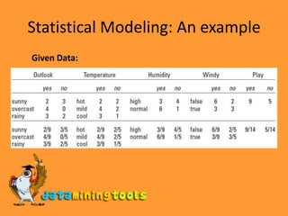
17. Statistical Modeling: An exampleDerivation using Bayes’ rule:Acc to Bayes’ rule, for a hypothesis H and evidence E that bears on that hypothesis, then P[H|E] = (P[E|H] x P[H]) / P[E]For our example hypothesis H is that play will be, say, yes and E is the particular combination of attribute values at handOutlook = sunny(E1)Temperature = cool (E2)Humidity = high(E3)Windy = True (E4)

18. Statistical Modeling: An exampleDerivation using Bayes’ rule:Now since E1, E2, E3 and E4 are independent therefore we have P[H|E] = (P[E1|H] x P[E2|H] x P[E3|H] x P[E4|H] x P[H] ) / P[E]Replacing values from the table we get, P[yes|E] = (2/9 x 3/9 x 3/9 x 3/9 x 9/14) / P[E]P[E] will be taken care of during normalization of P[yes|E] and P[No|E] This method is called as Naïve Bayes

19. Problem and Solution for Naïve BayesProblem:In case we have an attribute value (Ea)for which P[Ea|H] = 0, then irrespective of other attributes P[H|E] = 0Solution:We can add a constant to numerator and denominator, a technique called Laplace Estimator for example, P1 + P2 + P3 = 1:

20. Statistical Modeling: Dealing with missing attributesIncase an value is missing, say for attribute Ea in the given data set, we just don’t count it while calculating the P[Ea|H]Incase an attribute is missing in the instance to be classified, then its factor is not there in the expression for P[H|E], for example if outlook is missing then we will have:Likelihood of Yes = 3/9 x 3/9 x 3/9 x 9/14 = 0.0238 Likelihood of No = 1/5 x 4/5 x 3/5 x 5/14 = 0.0343

21. Statistical Modeling: Dealing with numerical attributesNumeric values are handled by assuming that they have :Normal probability distributionGaussian probability distributionFor a normal distribution we have: u = mean sigma = Standard deviation x = instance under consideration f(x) = contribution of to likelihood figures

22. Statistical Modeling: Dealing with numerical attributesAn example, we have the data:

23. Statistical Modeling: Dealing with numerical attributesSo here we have calculated the mean and standard deviation for numerical attributes like temperature and humidityFor temperature = 66So the contribution of temperature = 66 in P[yes|E] is 0.0340We do this similarly for other numerical attributes

24. Divide-and-Conquer: Constructing Decision TreesSteps to construct a decision tree recursively:Select an attribute to placed at root node and make one branch for each possible value Repeat the process recursively at each branch, using only those instances that reach the branch If at any time all instances at a node have the classification, stop developing that part of the treeProblem: How to decide which attribute to split on

25. Divide-and-Conquer: Constructing Decision TreesSteps to find the attribute to split on:We consider all the possible attributes as option and branch them according to different possible valuesNow for each possible attribute value we calculate Information and then find the Information gain for each attribute optionSelect that attribute for division which gives a Maximum Information GainDo this until each branch terminates at an attribute which gives Information = 0

26. Divide-and-Conquer: Constructing Decision TreesCalculation of Information and Gain:For data: (P1, P2, P3……Pn) such that P1 + P2 + P3 +……. +Pn = 1 Information(P1, P2 …..Pn) = -P1logP1 -P2logP2 – P3logP3 ……… -PnlogPnGain= Information before division – Information after division

27. Divide-and-Conquer: Constructing Decision TreesExample:Here we have consider eachattribute individuallyEach is divided into branches according to different possible values Below each branch the number ofclass is marked

28. Divide-and-Conquer: Constructing Decision TreesCalculations:Using the formulae for Information, initially we haveNumber of instances with class = Yes is 9 Number of instances with class = No is 5So we have P1 = 9/14 and P2 = 5/14Info[9/14, 5/14] = -9/14log(9/14) -5/14log(5/14) = 0.940 bitsNow for example lets consider Outlook attribute, we observe the following:

29. Divide-and-Conquer: Constructing Decision TreesExample Contd.Gain by using Outlook for division = info([9,5]) – info([2,3],[4,0],[3,2]) = 0.940 – 0.693 = 0.247 bitsGain (outlook) = 0.247 bits Gain (temperature) = 0.029 bits Gain (humidity) = 0.152 bits Gain (windy) = 0.048 bitsSo since Outlook gives maximum gain, we will use it for divisionAnd we repeat the steps for Outlook = Sunny and Rainy and stop for Overcast since we have Information = 0 for it

30. Divide-and-Conquer: Constructing Decision TreesHighly branching attributes: The problemIf we follow the previously subscribed method, it will always favor an attribute with the largest number of branchesIn extreme cases it will favor an attribute which has different value for each instance: Identification code

31. Divide-and-Conquer: Constructing Decision TreesHighly branching attributes: The problemInformation for such an attribute is 0info([0,1]) + info([0,1]) + info([0,1]) + …………. + info([0,1]) = 0It will hence have the maximum gain and will be chosen for branchingBut such an attribute is not good for predicting class of an unknown instance nor does it tells anything about the structure of divisionSo we use gain ratio to compensate for this

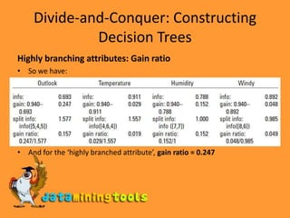
32. Divide-and-Conquer: Constructing Decision TreesHighly branching attributes: Gain ratioGain ratio = gain/split infoTo calculate split info, for each instance value we just consider the number of instances covered by each attribute value, irrespective of the classThen we calculate the split info, so for identification code with 14 different values we have:info([1,1,1,…..,1]) = -1/14 x log1/14 x 14 = 3.807For Outlook we will have the split info:info([5,4,5]) = -1/5 x log 1/5 -1/4 x log1/4 -1/5 x log 1/5 = 1.577

33. Divide-and-Conquer: Constructing Decision TreesHighly branching attributes: Gain ratioSo we have:And for the ‘highly branched attribute’, gain ratio = 0.247

34. Divide-and-Conquer: Constructing Decision TreesHighly branching attributes: Gain ratioThough the ‘highly branched attribute’ still have the maximum gain ratio, but its advantage is greatly reducedProblem with using gain ratio:In some situations the gain ratio modification overcompensates and can lead to preferring an attribute just because its intrinsic information is much lower than that for the other attributes. A standard fix is to choose the attribute that maximizes the gain ratio, provided that the information gain or that attribute is at least as great as the average information gain for all the attributes examined

35. Covering Algorithms: Constructing rulesApproach:Consider each class in turnSeek a way of covering all instances in it, excluding instances not belonging to this classIdentify a rule to do so This is called a covering approach because at each stage we identify a rule that covers some of the instances

36. Covering Algorithms: Constructing rulesVisualization: Rules for class = a: If x > 1.2 then class = a

37. If x > 1.2 and y > 2.6 then class = a

38. If x > 1.2 and y > 2.6 then class = a If x > 1.4 and y < 2.4 then class = a

39. Covering Algorithms: Constructing rulesRules Vs Trees:Covering algorithm covers only a single class at a time whereas division takes all the classes in account as decision trees creates a combines concept descriptionProblem of replicated sub trees is avoided in rulesTree for the previous problem:

40. Covering Algorithms: Constructing rulesPRISM Algorithm: A simple covering algorithmInstance space after addition of rules:

41. Covering Algorithms: Constructing rulesPRISM Algorithm: Criteria to select an attribute for divisionInclude as many instances of the desired class and exclude as many instances of other class as possibleIf a new rule covers t instances of which p are positive examples of the class and t-p are instances of other classes i.e errors, then try to maximize p/t

42. Covering Algorithms: Constructing rulesPRISM Algorithm: Example data

43. Covering Algorithms: Constructing rulesPRISM Algorithm: In actionWe start with the class = hard and have the following rule:If ? Then recommendation = hardHere ? represents an unknown ruleFor unknown we have nine choices:

44. Covering Algorithms: Constructing rulesPRISM Algorithm: In actionHere the maximum t/p ratio is for astigmatism = yes (choosing randomly between equivalent option in case there coverage is also same)So we get the rule:If astigmatism = yes then recommendation = hardWe wont stop at this rule as this rule gives only 4 correct results out of 12 instances it coversWe remove the correct instances of the above rule from our example set and start with the rule:If astigmatism = yes and ? then recommendation = hard

45. Covering Algorithms: Constructing rulesPRISM Algorithm: In actionNow we have the data as:

46. Covering Algorithms: Constructing rulesPRISM Algorithm: In actionAnd the choices for this data is:We choose tear production rate = normal which has highest t/p

47. Covering Algorithms: Constructing rulesPRISM Algorithm: In actionSo we have the rule:If astigmatism = yes and tear production rate = normal then recommendation = hardAgain, we remove matched instances, now we have the data:

48. Covering Algorithms: Constructing rulesPRISM Algorithm: In actionNow again using t/p we finally have the rule (based on maximum coverage):If astigmatism = yes and tear production rate = normal and spectacle prescription = myope then recommendation = hard And so on. …..

49. Covering Algorithms: Constructing rulesPRISM Algorithm: Pseudo Code

50. Covering Algorithms: Constructing rulesRules Vs decision listsThe rules produced, for example by PRISM algorithm, are not necessarily to be interpreted in order like decision listsThere is no order in which class should be considered while generating rules Using rules for classification, one instance may receive multiple receive multiple classification or no classification at allIn such cases go for the rule with maximum coverage and training examples respecitivelyThese difficulties are not there with decision lists as they are to be interpreted in order and have a default rule at the end

51. Mining Association RulesDefinition:An association rule can predict any number of attributes and also any combination of attributesParameter for selecting an Association Rule:Coverage: The number of instances they predict correctlyAccuracy: The ratio of coverageand total number of instances the rule is applicableWe want association rule with high coverage and a minimum specified accuracy

52. Mining Association RulesTerminology:Item – set: A combination of attributesItem: An attribute – value pairAn example:For the weather data we have a table with each column containing an item – set having different number of attributesWith each entry the coverage is also givenThe table is not complete, just gives us a good idea

53. Mining Association Rules

54. Mining Association RulesGenerating Association rules:We need to specify a minimum coverage and accuracy for the rules to be generated before handSteps:Generate the item setsEach item set can be permuted to generate a number of rulesFor each rule check if the coverage and accuracy is appropriate This is how we generate association rules

55. Mining Association RulesGenerating Association rules:For example if we take the item set:humidity = normal, windy = false, play = yesThis gives seven potential rules (with accuracy):

56. Linear modelsWe will look at methods to deal with the prediction of numerical quantitiesWe will see how to use numerical methods for classification

57. Linear modelsNumerical Prediction: Linear regressionLinear regression is a technique to predict numerical quantitiesHere we express the class (a numerical quantity) as a linear combination of attributes with predetermined weightsFor example if we have attributes a1,a2,a3…….,akx = (w0) + (w1)x(a1) + (w2)x(a2) + …… + (wk)x(ak) Here x represents the predicted class and w0,w1……,wk are the predetermined weights

58. Linear modelsNumerical Prediction: Linear regressionThe weights are calculated by using the training setTo choose optimum weights we select the weights with minimum square sum:

59. Linear modelsLinear classification: Multi response linear regression For each class we use linear regression to get a linear expression When the instance belongs to the class output is 1, otherwise 0Now for an unclassified instance we use the expression for each class and get an outputThe class expression giving the maximum output is selected as the classified classThis method has the drawbacks that values produced are not proper probabilities

60. Linear modelsLinear classification: Logistic regressionTo get the output as proper probabilities in the range 0 to 1 we use logistic regressionHere the output y is defined as: y = 1/(1+e^(-x))x = (w0) + (w1)x(a1) + (w2)x(a2) + …… + (wk)x(ak)So the output y will lie in the range (0,1]

61. Linear modelsLinear classification: Logistic regressionTo select appropriate weights for the expression of x, we maximize:To generalize Logistic regression we can use do the calculation like we did in Multi response linear regression Again the problem with this approach is that the probabilities of different classes do not sum up to 1

62. Linear modelsLinear classification using the perceptronIf instances belonging to different classes can be divided in the instance space by using hyper planes, then they are called linearly separableIf instances are linearly separable then we can use perceptron learning rule for classification Steps:Lets assume that we have only 2 classesThe equation of hyper plane is (a0 = 1): (w0)(a0) + (w1)(a1) + (w2)(a2) +…….. + (wk)(ak) = 0

63. Linear modelsLinear classification using the perceptronSteps (contd.):If the sum (mentioned in previous step) is greater than 0 than we have first class else the second oneThe algorithm to get the weight and hence the equation of dividing hyper plane (or the perceptron)is:

64. Instance-based learningGeneral steps:No preprocessing of training sets, just store the training instances as it isTo classify a new instance calculate its distance with every stored training instanceThe unclassified instance is allotted the class of the instance which has the minimum distance from it

65. Instance-based learningThe distance functionThe distance function we use depends on our applicationSome of the popular distance functions are: Euclidian distance, Manhattan distance metric etc.The most popular distance metric is Euclidian distance (between teo instances) given by: K is the number of attributes

66. Instance-based learningNormalization of data:We normalize attributes such that they lie in the range [0,1], by using the formulae:Missing attributes:In case of nominal attributes, if any of the two attributes are missing or if the attributes are different, the distance is taken as 1 In nominal attributes, if both are missing than difference is 1. If only one attribute is missing than the difference is the either the normalized value of given attribute or one minus that size, which ever is bigger

67. Instance-based learningFinding nearest neighbors efficiently:Finding nearest neighbor by calculating distance with every attribute of each instance if linearWe make this faster by using kd-treesKD-Trees:They are binary trees that divide the input space with a hyper plane and then split each partition again, recursivelyIt stores the points in k dimensional space, k being the number of attributes

68. Instance-based learningFinding nearest neighbors efficiently:

69. Instance-based learningFinding nearest neighbors efficiently:Here we see a kd tree and the instances and splits with k=2As you can see not all child nodes are developed to the same depthWe have mentioned the axis along which the division has been done (v or h in this case)Steps to find the nearest neighbor:Construct the kd tree (explained later)Now start from the root node and comparing the appropriate attribute (based on the axis along which the division has been done), move to left or the right sub-tree

70. Instance-based learningSteps to find the nearest neighbor (contd.):Repeat this step recursively till you reach a node which is either a leaf node or has no appropriate leaf node (left or right)Now you have find the region to which this new instance belongYou also have a probable nearest neighbor in the form of the regions leaf node (or immediate neighbor)Calculate the distance of the instance with the probable nearest neighbor. Any closer instance will lie in a circle with radius equal to this distance

71. Instance-based learningFinding nearest neighbors efficiently:Steps to find the nearest neighbor (contd.):Now we will move redo our recursive trace looking for an instance which is closer to put unclassified instance than the probable nearest neighbor we haveWe start with the immediate neighbor, if it lies in the circle than we will have to consider it and all its child nodes (if any)If condition of previous step is not true then we check the siblings of the parent of our probable nearest neighborWe repeat these steps till we reach the rootIn case we find instance(s) which are nearer, we update the nearest neighbor

72. Instance-based learningSteps to find the nearest neighbor (contd.):

73. Instance-based learningConstruction of KD tree:We need to figure out two things to construct a kd tree:Along which dimension to make the cutWhich instance to use to make the cutDeciding the dimension to make the cut:We calculate the variance along each axisThe division is done perpendicular to the axis with minimum varianceDeciding the instance to be used for division:Just take the median as the point of division So we repeat these steps recursively till all the points are exhausted

74. ClusteringClustering techniques apply when rather than predicting the class, we just want the instances to be divided into natural groupIterative instance based learning: k-meansHere k represents the number of clustersThe instance space is divided in to k clustersK-means forms the cluster so as the sum of square distances of instances from there cluster center is minimum