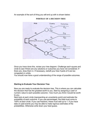
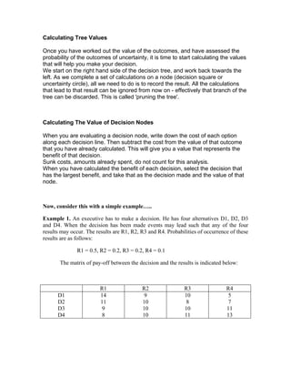
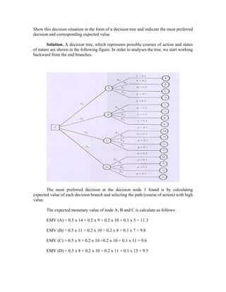
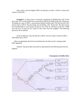
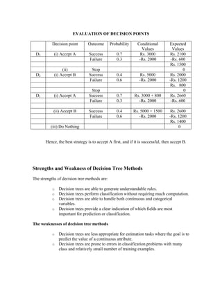
Unit 4
DECISION ANALYSIS
Lesson 37
Learning objectives:
• To learn how to use decision trees.
• To structure complex decision making problems.
• To analyze the above problems.
• To find out limitations & advantages of decision tree analysis.
Helping you to think your way to an excellent life!
Decision Theory and Decision Trees
Hello Students,
Decision trees are excellent tools for making financial or number based decisions
where a lot of complex information needs to be taken into account. They provide
an effective structure in which alternative decisions and the implications of taking
those decisions can be laid down and evaluated. They also help you to form an
accurate, balanced picture of the risks and rewards that can result from a
particular choice.
What is a decision tree ?
Decision tree is a classifier in the form of a tree structure.
So far, the decision criteria are applicable to situations where we have to
make a single decision. There is another technique for analyzing a
decision situation. A decision tree is a schematic diagram consisting of
nodes and branches. There are some advantages of using this technique:
1. It provides a pictorial representation of the sequential decision
process. Each process requires one payoff table.
2. It is easier to compute the expected value (opportunity loss). We
can do them directly on the tree diagram.
3. More than one decision maker can be easily involved with the
decision processes.
There are only three rules governing the construction of a decision tree:
branches emanating from a decision node reflect the
alternative decisions possible at that point.
If a decision situation requires a series of decisions, then a payoff table
approach cannot accommodate the multiple layers of decision - making. A
decision tree approach becomes the best method. However, a tree diagram
will contain nothing but more squares (decision nodes). We can still apply
the expected value criterion at each decision node from the right to the left
of a tree diagram (backward process).
A decision tree can be used to classify an example by starting at the root of the tree and
moving through it until an event node occurs, which provides the classification of the
instance.
Decision tree induction is a typical inductive approach to learn knowledge on
classification. The key requirements to do mining with decision trees are:
o Attribute-value description: object or case must be expressible in terms of
a fixed collection of properties or attributes. This means that we need to
discretize continuous attributes, or this must have been provided in the
algorithm.
o Predefined classes (target attribute values): The categories to which
examples are to be assigned must have been established beforehand
(supervised data).
o Discrete classes: A case does or does not belong to a particular class, and
there must be more cases than classes.
o Sufficient data: Usually hundreds or even thousands of training cases.
How to Draw a Decision Tree?
You start a decision tree with a decision that needs to be made. This decision is
represented by a small square towards the left of a large piece of paper. From
this box draw out lines towards the right for each possible solution, and write that
solution along the line. Keep the lines apart as far as possible so that you can
expand your thoughts.
At the end of each solution line, consider the results. If the result of taking that
decision is uncertain, draw a small circle. If the result is another decision that
needs to be made, draw another square. Squares represent decisions, circles
represent uncertainty or random factors. Write the decision or factor to be
considered above the square or circle. If you have completed the solution at the
end of the line, just leave it blank.
Starting from the new decision squares on your diagram, draw out lines
representing the options that could be taken. From the circles draw out lines
representing possible outcomes. Again mark a brief note on the line saying what
it means. Keep on doing this until you have drawn down as many of the possible
outcomes and decisions as you can see leading on from your original decision.
An example of the sort of thing you will end up with is shown below:
PORTRAY OF A DECISION TREE
Once you have done this, review your tree diagram. Challenge each square and
circle to see if there are any solutions or outcomes you have not considered. If
there are, draw them in. If necessary, redraft your tree if parts of it are too
congested or untidy.
You should now have a good understanding of the range of possible outcomes.
Starting to Evaluate Your Decision Tree
Now you are ready to evaluate the decision tree. This is where you can calculate
the decision that has the greatest worth to you. Start by assigning a cash or
numeric value to each possible outcome - how much you think it would be worth
to you.
Next look at each circle (representing an uncertainty point) and estimate the
probability of each outcome. If you use percentages, the total must come to
100% at each circle. If you use fractions, these must add up to 1. If you have
data on past events you may be able to make rigorous estimates of the
probabilities. Otherwise write down your best guess.
Calculating Tree Values
Once you have worked out the value of the outcomes, and have assessed the
probability of the outcomes of uncertainty, it is time to start calculating the values
that will help you make your decision.
We start on the right hand side of the decision tree, and work back towards the
left. As we complete a set of calculations on a node (decision square or
uncertainty circle), all we need to do is to record the result. All the calculations
that lead to that result can be ignored from now on - effectively that branch of the
tree can be discarded. This is called 'pruning the tree'.
Calculating The Value of Decision Nodes
When you are evaluating a decision node, write down the cost of each option
along each decision line. Then subtract the cost from the value of that outcome
that you have already calculated. This will give you a value that represents the
benefit of that decision.
Sunk costs, amounts already spent, do not count for this analysis.
When you have calculated the benefit of each decision, select the decision that
has the largest benefit, and take that as the decision made and the value of that
node.
Now, consider this with a simple example…..
Example 1. An executive has to make a decision. He has four alternatives D1, D2, D3
and D4. When the decision has been made events may lead such that any of the four
results may occur. The results are R1, R2, R3 and R4. Probabilities of occurrence of these
results are as follows:
R1 = 0.5, R2 = 0.2, R3 = 0.2, R4 = 0.1
The matrix of pay-off between the decision and the results is indicated below:
R1 R2 R3 R4
D1
D2
D3
D4
14
11
9
8
9
10
10
10
10
8
10
11
5
7
11
13
Show this decision situation in the form of a decision tree and indicate the most preferred
decision and corresponding expected value.
Solution. A decision tree, which represents possible courses of action and states
of nature are shown in the following figure. In order to analyses the tree, we start working
backward from the end branches.
The most preferred decision at the decision node 1 found is by calculating
expected value of each decision branch and selecting the path (course of action) with high
value.
The expected monetary value of node A, B and C is calculate as follows:
EMV (A) = 0.5 x 14 + 0.2 x 9 + 0.2 x 10 + 0.1 x 5 = 11.3
EMV (B) = 0.5 x 11 + 0.2 x 10 + 0.2 x 8 + 0.1 x 7 = 9.8
EMV (C) = 0.5 x 9 + 0.2 x 10 +0.2 x 10 + 0.1 x 11 = 9.6
EMV (D) = 0.5 x 8 + 0.2 x 10 + 0.2 x 11 + 0.1 x 13 = 9.5
Since node A has the highest EMV, the decision at node 1 will be to choose the
course of action D4.
Example 2. A farm owner is seriously considering of drilling farm well. In the
past, only 70% of wells drilled were successful at 200 feet of depth in the area. Moreover,
on finding no water at 200 ft., some persons drilled it further up to 250 feet but only 20%
struck water at 250 ft. The prevailing cost of drilling is Rs. 50 per feet. The farm owner
has estimated that in case he loss not get his own well, he will have to pay Rs. 15,000
over the next 10 years (in PV terms) to buy water from the neighbor. The following
decisions can be optimal:
(i) do not drill any well, (ii) drill up to 200 ft. (iii) if no water is found at 200 ft.,
drill further up to 250 ft.
Draw an appropriate decision tree and determine the farm owner’s strategy under
EMV approach.
Solution. The given data can easily be represented by the following decision tree
diagram.
Consequence of outflow (Rs.)
There are two decision points in the tree indicated by 1 and 2. In order to decide
between the two basis alternatives, we have to fold back (backward induction) the tree
from the decision point 2, using EMV as criterion:
EVALUATION OF DECISION POINTS
Decision point
State of
Nature
Probability
Cash outflows
Expected cash
Outflow
Decision at point D2
1. Drill up to
250 fit.
Water struck 0.2 Rs. 12,5000 Rs. 2,500
No water struck 0.8 27,500 22,000
EMV (outflows) = 24,500
2. Do not drill
up to 250 ft.
EMV (outflow) = Rs. 25,000
The decision at D2 is : Drill up to 250 feet.
Decision at point D2
1. Drill up to
200 ft.
Water struck 0.7 Rs. 10,000 Rs. 7,000
Not water
struck
0.3 24,500 7,350
EMV (outflow) = Rs. 14,350
2. Do not drill
up to 200 ft.
EMV (outflow) = Rs. 15,000
The decision at D1 is : Drill up to 200 ft.
Thus the optimal strategy for the farm-owner is to drill the well up to 200 ft. and
if no water is struck, then further drill it up to 250 ft.
Example 3. A businessman has two independent investments A and B available to
him; but he lacks the capital to undertake both of them simultaneously. He can choose to
take A first and then stop, or if A is successful then take B, or vice versa. The probability
of success of A is 0.7, while for B it is 0’4. Both investments require an initial capital
outlay of Rs. 2,000, and both return nothing if the venture is unsuccessful. Successful
competitions of A will return Rs. 3,000 (over cost), and successful completion of B will
return Rs. 5,000 (over cost). Draw the decision tree and determine the best strategy.
Solution. The appropriate decision tree is shown below:
There are three decision points in the above decision tree indicated by D1, D2 and D3.
EVALUATION OF DECISION POINTS
Decision point Outcome Probability Conditional
Values
Expected
Values
D3 (i) Accept A Success 0.7 Rs. 3000 Rs. 2100
Failure 0.3 -Rs. 2000 -Rs. 600
Rs. 1500
(ii) Stop 0
D2 (i) Accept B Success 0.4 Rs. 5000 Rs. 2000
Failure 0.6 -Rs. 2000 -Rs. 1200
Rs. 800
Stop 0
D1 (i) Accept A Success 0.7 Rs. 3000 + 800 Rs. 2660
Failure 0.3 -Rs. 2000 -Rs. 600
(ii) Accept B Success 0.4 Rs. 5000 + 1500 Rs. 2600
Failure 0.6 -Rs. 2000 -Rs. 1200
Rs. 1400
(iii) Do Nothing 0
Hence, the best strategy is to accept A first, and if it is successful, then accept B.
Strengths and Weakness of Decision Tree Methods
The strengths of decision tree methods are:
o Decision trees are able to generate understandable rules.
o Decision trees perform classification without requiring much computation.
o Decision trees are able to handle both continuous and categorical
variables.
o Decision trees provide a clear indication of which fields are most
important for prediction or classification.
The weaknesses of decision tree methods
o Decision trees are less appropriate for estimation tasks where the goal is to
predict the value of a continuous attribute.
o Decision trees are prone to errors in classification problems with many
class and relatively small number of training examples.
o Decision tree can be computationally expensive to train. The process of
growing a decision tree is computationally expensive. At each node, each
candidate splitting field must be sorted before its best split can be found.
In some algorithms, combinations of fields are used and a search must be
made for optimal combining weights. Pruning algorithms can also be
expensive since many candidate sub-trees must be formed and compared.
o Decision trees do not treat well non-rectangular regions. Most decision-
tree algorithms only examine a single field at a time. This leads to
rectangular classification boxes that may not correspond well with the
actual distribution of records in the decision space.
In this lecture you must have got a hang as to how decision tree analysis is used to
arrive at business decisions.
Summary
Decision trees provide an effective method of decision making because they:
• clearly lay out the problem so that all choices can be viewed, discussed
and challenged
• provide a framework to quantify of the values of outcomes and the
probabilities of achieving them
• help us to make the best decisions on the basis of our existing information
and best guesses.
As with all decision-making methods, though, decision tree analysis should be
used in conjunction with common sense. They are just one important part of your
decision-making tool kit.

Decision theory & decisiontrees

  • 1.
    Unit 4 DECISION ANALYSIS Lesson37 Learning objectives: • To learn how to use decision trees. • To structure complex decision making problems. • To analyze the above problems. • To find out limitations & advantages of decision tree analysis. Helping you to think your way to an excellent life! Decision Theory and Decision Trees Hello Students, Decision trees are excellent tools for making financial or number based decisions where a lot of complex information needs to be taken into account. They provide an effective structure in which alternative decisions and the implications of taking
  • 2.
    those decisions canbe laid down and evaluated. They also help you to form an accurate, balanced picture of the risks and rewards that can result from a particular choice. What is a decision tree ? Decision tree is a classifier in the form of a tree structure. So far, the decision criteria are applicable to situations where we have to make a single decision. There is another technique for analyzing a decision situation. A decision tree is a schematic diagram consisting of nodes and branches. There are some advantages of using this technique: 1. It provides a pictorial representation of the sequential decision process. Each process requires one payoff table. 2. It is easier to compute the expected value (opportunity loss). We can do them directly on the tree diagram. 3. More than one decision maker can be easily involved with the decision processes. There are only three rules governing the construction of a decision tree: branches emanating from a decision node reflect the alternative decisions possible at that point. If a decision situation requires a series of decisions, then a payoff table approach cannot accommodate the multiple layers of decision - making. A decision tree approach becomes the best method. However, a tree diagram will contain nothing but more squares (decision nodes). We can still apply the expected value criterion at each decision node from the right to the left of a tree diagram (backward process).
  • 3.
    A decision treecan be used to classify an example by starting at the root of the tree and moving through it until an event node occurs, which provides the classification of the instance. Decision tree induction is a typical inductive approach to learn knowledge on classification. The key requirements to do mining with decision trees are: o Attribute-value description: object or case must be expressible in terms of a fixed collection of properties or attributes. This means that we need to discretize continuous attributes, or this must have been provided in the algorithm. o Predefined classes (target attribute values): The categories to which examples are to be assigned must have been established beforehand (supervised data). o Discrete classes: A case does or does not belong to a particular class, and there must be more cases than classes. o Sufficient data: Usually hundreds or even thousands of training cases. How to Draw a Decision Tree? You start a decision tree with a decision that needs to be made. This decision is represented by a small square towards the left of a large piece of paper. From this box draw out lines towards the right for each possible solution, and write that solution along the line. Keep the lines apart as far as possible so that you can expand your thoughts. At the end of each solution line, consider the results. If the result of taking that decision is uncertain, draw a small circle. If the result is another decision that needs to be made, draw another square. Squares represent decisions, circles represent uncertainty or random factors. Write the decision or factor to be considered above the square or circle. If you have completed the solution at the end of the line, just leave it blank. Starting from the new decision squares on your diagram, draw out lines representing the options that could be taken. From the circles draw out lines representing possible outcomes. Again mark a brief note on the line saying what it means. Keep on doing this until you have drawn down as many of the possible outcomes and decisions as you can see leading on from your original decision.
  • 4.
    An example ofthe sort of thing you will end up with is shown below: PORTRAY OF A DECISION TREE Once you have done this, review your tree diagram. Challenge each square and circle to see if there are any solutions or outcomes you have not considered. If there are, draw them in. If necessary, redraft your tree if parts of it are too congested or untidy. You should now have a good understanding of the range of possible outcomes. Starting to Evaluate Your Decision Tree Now you are ready to evaluate the decision tree. This is where you can calculate the decision that has the greatest worth to you. Start by assigning a cash or numeric value to each possible outcome - how much you think it would be worth to you. Next look at each circle (representing an uncertainty point) and estimate the probability of each outcome. If you use percentages, the total must come to 100% at each circle. If you use fractions, these must add up to 1. If you have data on past events you may be able to make rigorous estimates of the probabilities. Otherwise write down your best guess.
  • 5.
    Calculating Tree Values Onceyou have worked out the value of the outcomes, and have assessed the probability of the outcomes of uncertainty, it is time to start calculating the values that will help you make your decision. We start on the right hand side of the decision tree, and work back towards the left. As we complete a set of calculations on a node (decision square or uncertainty circle), all we need to do is to record the result. All the calculations that lead to that result can be ignored from now on - effectively that branch of the tree can be discarded. This is called 'pruning the tree'. Calculating The Value of Decision Nodes When you are evaluating a decision node, write down the cost of each option along each decision line. Then subtract the cost from the value of that outcome that you have already calculated. This will give you a value that represents the benefit of that decision. Sunk costs, amounts already spent, do not count for this analysis. When you have calculated the benefit of each decision, select the decision that has the largest benefit, and take that as the decision made and the value of that node. Now, consider this with a simple example….. Example 1. An executive has to make a decision. He has four alternatives D1, D2, D3 and D4. When the decision has been made events may lead such that any of the four results may occur. The results are R1, R2, R3 and R4. Probabilities of occurrence of these results are as follows: R1 = 0.5, R2 = 0.2, R3 = 0.2, R4 = 0.1 The matrix of pay-off between the decision and the results is indicated below: R1 R2 R3 R4 D1 D2 D3 D4 14 11 9 8 9 10 10 10 10 8 10 11 5 7 11 13
  • 6.
    Show this decisionsituation in the form of a decision tree and indicate the most preferred decision and corresponding expected value. Solution. A decision tree, which represents possible courses of action and states of nature are shown in the following figure. In order to analyses the tree, we start working backward from the end branches. The most preferred decision at the decision node 1 found is by calculating expected value of each decision branch and selecting the path (course of action) with high value. The expected monetary value of node A, B and C is calculate as follows: EMV (A) = 0.5 x 14 + 0.2 x 9 + 0.2 x 10 + 0.1 x 5 = 11.3 EMV (B) = 0.5 x 11 + 0.2 x 10 + 0.2 x 8 + 0.1 x 7 = 9.8 EMV (C) = 0.5 x 9 + 0.2 x 10 +0.2 x 10 + 0.1 x 11 = 9.6 EMV (D) = 0.5 x 8 + 0.2 x 10 + 0.2 x 11 + 0.1 x 13 = 9.5
  • 7.
    Since node Ahas the highest EMV, the decision at node 1 will be to choose the course of action D4. Example 2. A farm owner is seriously considering of drilling farm well. In the past, only 70% of wells drilled were successful at 200 feet of depth in the area. Moreover, on finding no water at 200 ft., some persons drilled it further up to 250 feet but only 20% struck water at 250 ft. The prevailing cost of drilling is Rs. 50 per feet. The farm owner has estimated that in case he loss not get his own well, he will have to pay Rs. 15,000 over the next 10 years (in PV terms) to buy water from the neighbor. The following decisions can be optimal: (i) do not drill any well, (ii) drill up to 200 ft. (iii) if no water is found at 200 ft., drill further up to 250 ft. Draw an appropriate decision tree and determine the farm owner’s strategy under EMV approach. Solution. The given data can easily be represented by the following decision tree diagram. Consequence of outflow (Rs.)
  • 8.
    There are twodecision points in the tree indicated by 1 and 2. In order to decide between the two basis alternatives, we have to fold back (backward induction) the tree from the decision point 2, using EMV as criterion: EVALUATION OF DECISION POINTS Decision point State of Nature Probability Cash outflows Expected cash Outflow Decision at point D2 1. Drill up to 250 fit. Water struck 0.2 Rs. 12,5000 Rs. 2,500 No water struck 0.8 27,500 22,000 EMV (outflows) = 24,500 2. Do not drill up to 250 ft. EMV (outflow) = Rs. 25,000 The decision at D2 is : Drill up to 250 feet. Decision at point D2 1. Drill up to 200 ft. Water struck 0.7 Rs. 10,000 Rs. 7,000 Not water struck 0.3 24,500 7,350 EMV (outflow) = Rs. 14,350 2. Do not drill up to 200 ft. EMV (outflow) = Rs. 15,000 The decision at D1 is : Drill up to 200 ft. Thus the optimal strategy for the farm-owner is to drill the well up to 200 ft. and if no water is struck, then further drill it up to 250 ft. Example 3. A businessman has two independent investments A and B available to him; but he lacks the capital to undertake both of them simultaneously. He can choose to
  • 9.
    take A firstand then stop, or if A is successful then take B, or vice versa. The probability of success of A is 0.7, while for B it is 0’4. Both investments require an initial capital outlay of Rs. 2,000, and both return nothing if the venture is unsuccessful. Successful competitions of A will return Rs. 3,000 (over cost), and successful completion of B will return Rs. 5,000 (over cost). Draw the decision tree and determine the best strategy. Solution. The appropriate decision tree is shown below: There are three decision points in the above decision tree indicated by D1, D2 and D3.
  • 10.
    EVALUATION OF DECISIONPOINTS Decision point Outcome Probability Conditional Values Expected Values D3 (i) Accept A Success 0.7 Rs. 3000 Rs. 2100 Failure 0.3 -Rs. 2000 -Rs. 600 Rs. 1500 (ii) Stop 0 D2 (i) Accept B Success 0.4 Rs. 5000 Rs. 2000 Failure 0.6 -Rs. 2000 -Rs. 1200 Rs. 800 Stop 0 D1 (i) Accept A Success 0.7 Rs. 3000 + 800 Rs. 2660 Failure 0.3 -Rs. 2000 -Rs. 600 (ii) Accept B Success 0.4 Rs. 5000 + 1500 Rs. 2600 Failure 0.6 -Rs. 2000 -Rs. 1200 Rs. 1400 (iii) Do Nothing 0 Hence, the best strategy is to accept A first, and if it is successful, then accept B. Strengths and Weakness of Decision Tree Methods The strengths of decision tree methods are: o Decision trees are able to generate understandable rules. o Decision trees perform classification without requiring much computation. o Decision trees are able to handle both continuous and categorical variables. o Decision trees provide a clear indication of which fields are most important for prediction or classification. The weaknesses of decision tree methods o Decision trees are less appropriate for estimation tasks where the goal is to predict the value of a continuous attribute. o Decision trees are prone to errors in classification problems with many class and relatively small number of training examples.
  • 11.
    o Decision treecan be computationally expensive to train. The process of growing a decision tree is computationally expensive. At each node, each candidate splitting field must be sorted before its best split can be found. In some algorithms, combinations of fields are used and a search must be made for optimal combining weights. Pruning algorithms can also be expensive since many candidate sub-trees must be formed and compared. o Decision trees do not treat well non-rectangular regions. Most decision- tree algorithms only examine a single field at a time. This leads to rectangular classification boxes that may not correspond well with the actual distribution of records in the decision space. In this lecture you must have got a hang as to how decision tree analysis is used to arrive at business decisions. Summary Decision trees provide an effective method of decision making because they: • clearly lay out the problem so that all choices can be viewed, discussed and challenged • provide a framework to quantify of the values of outcomes and the probabilities of achieving them • help us to make the best decisions on the basis of our existing information and best guesses. As with all decision-making methods, though, decision tree analysis should be used in conjunction with common sense. They are just one important part of your decision-making tool kit.