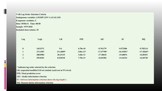
Downloaded 266 times


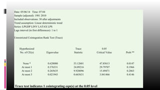
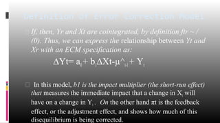
![Vector Error Correction Estimates
Date: 05/26/14 Time: 22:36
Sample (adjusted): 1981 2010
Included observations: 30 after adjustments
Standard errors in ( ) & t-statistics in [ ]
Cointegrating Eq: CointEq1
LPGDP(-1) 1.000000
LINV(-1) -4.620559
(0.47459)
[-9.73587]
LATAX(-1) -3.350165
(1.20384)
[-2.78289]
LPS(-1) 1.274220
(0.49822)
[ 2.55755]
C -3.861790
Error Correction: D(LPGDP) D(LINV) D(LATAX) D(LPS)
CointEq1 -0.011599 0.167417 -0.004750 -0.060848
(0.02160) (0.04974) (0.02840) (0.03017)
[-0.53695] [ 3.36570] [-0.16725] [-2.01682]](https://image.slidesharecdn.com/3cointegrationpresentationnrgs-140822082057-phpapp01/85/Co-integration-14-320.jpg)
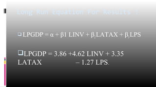


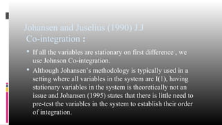
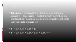
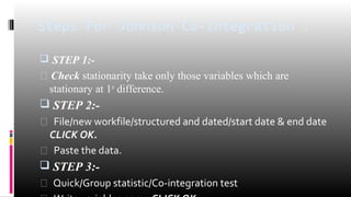
The document discusses the concept of cointegration and its various approaches, particularly focusing on the Engle-Granger and Johansen-Juselius methods. It outlines the conditions necessary for cointegration, interpretations of the Error Correction Model (ECM), and provides steps for conducting estimations using these methodologies. Additionally, it includes examples, definitions, and references for further reading on the subject.