Note

1. CHAPTER VI: Time Series Analysis
6.1 The concept of stationarity
Definition: A series t
Y is said to be weakly or covariance stationary if:
i) t
E(Y )   (constant)
ii) 2 2
t t
var(Y ) E(Y )
      (finite (and constant) variance)
iii) t t s t t s
cov(Y ,Y ) E{(Y )(Y )} (s)
 
    
The conditions imply that the mean, variance and the covariance of the process are
independent of time. Condition (iii) states that the covariance between t
Y and t s
Y
does not depend on t – it is rather a function of the time lag between the two
observations (s), that is, the covariance is a function of how far apart the two
observations are. For example, the covariance between t
Y and t 1
Y is the same as the
covariance between t 6
Y  and t 7
Y  .
(s)
 is known as the autocovariance function (since it is the covariance of t
Y with its
own previous (or lagged) values). When s = 0, the autocovariance function is simply
the variance of t
Y . The autocovariances are not as such particularly useful measures
of the relationship between t
Y and its previous values since they depend on the units of
measurement, and hence the values that they take have no immediate interpretation.
It is thus more convenient to work with autocorrelations:
(s)
(s) s 1, 2, 3, . . .
(0)

  

The series (s)
 has the standard property of correlation coefficients, that is, the values
are bounded between – 1 and + 1, inclusive ( 1 (s) 1
     ). If s = 0, we get the
correlation of t
Y with itself (which is of course +1). The plot of (s)
 against
s 1, 2, 3, . . .
 is called the autocorrelation function (ACF) or correlogram.
Definition: A series t
u is said to be white noise if:
i) t
E(u ) 0

ii) 2
t u
var(u )    
iii) t t s
cov(u ,u ) 0 s 0
  
Thus, a white noise process has zero mean, constant variance (independent of t), and
zero autocovariances. The last condition implies that each observation is uncorrelated
with all other values in the sequence.
6.2 Autoregressive processes and stationarity
An autoregressive model is a model where the current value of a variable t
Y depends
upon only the values that the variable took in previous periods plus an error term. An
autoregressive process of order p, denoted by AR(p) , can be expressed as:

2. 80
CHAPTER VI: Time Series Analysis
t 1 t 1 2 t 2 p t p t
Y Y Y . . . Y u
  
      ………………… (1)
where t
u is a white noise disturbance term.
Stationarity is a desirable property of an AR model for several reasons. One important
reason is that a non-stationary AR process exhibits the property that previous values of
the white noise error term will have a non-declining effect on the current value of t
Y as
time progresses. In contrast, the autocovariances (and hence, the autocorrelations) of a
stationary AR process will decline eventually as the lag length is increased (the ACF
will decay geometrically to zero).
Example: Consider the autoregressive model of order one ( AR(1) model):
t t 1 t
Y Y u

  
where t
u is a white noise disturbance term. It can be shown that the autocovariance
function of this process is:
2
t t s
s
(s) cov(Y ,Y ) s 1, 2, 3, . . .

     
i) If | | 1
  , then the term s
 will tend to infinity as s tend to infinity - the
autocovariance function of the process will also tend to infinity rather than
declining. For example, let 4
  :
 2 2
1
(1) (4) 4
    
 2 2
2
(2) (4) 16
    
 2 2
3
(3) (4) 64
    
 2 2
4
(4) (4) 256
    
We can clearly see that the autocovariance function keeps on increasing as the time lag
(s) increases. Thus, the process is non-stationary.
ii) If 1
  , then 2
(s)
   (constant) for all s 1, 2, 3, . . .
 ., that is, the
autocovariance function will never decline however large the lag length is. Thus,
the process is non-stationary.
iii) If | | 1
  , then the autocovariance function will tend to zero as the lag length (s)
increases. For example, let 1/5
  :
 2 2
1
(1) (1/5) /5
   
 2 2
2
(2) (1/5) / 25
   
 2 2
3
(3) (1/5) /125
   
 2 2
4
(4) (1/5) /625
   
We can clearly see that as s   , (s) 0
  , that is, the autocovariance function decays
to zero when the time lag (s) becomes very large. Thus, the process is stationary.
When 1
  , the process is said to be a random-walk process:
t t 1 t
Y Y u

 

3. 81 Applied Econometrics for Accounting and Finance
where t
u is white noise as usual. One key feature (trait) of random walks is that the
most recently observed value of the variable is the best forecaster of future values.
6.3 Characteristic equation
The backward shift operator or lag operator Z is defined as:
p
t t p
Z Y Y p 1, 2, 3, . . .

 
When p = 1, for example, the variable is shifted one period back: 1
t t t 1
Z Y ZY Y
  .
Similarly, 2
t t 2
Z Y Y
 , 3
t t 3
Z Y Y
 , etc.
Using the backward shift operator, the AR(p) model can be written as:
t 1 t 1 2 t 2 p t p t
Y Y Y . . . Y u
  
     
2 p
t 1 t 2 t p t t
Y ZY Z Y . . . Z Y u
      
2 p
1 2 p t t
(1 Z Z . . . Z )Y u
     
t t
a(Z)Y u
 
The equation:
a(Z) 0
 2 p
1 2 p
1 Z Z . . . Z 0
     
is the so-called the characteristic equation of the process. The notion of a
characteristic equation comes from the fact that its roots determine the characteristics of
the process t
Y . The AR(p) process is stationary if the roots of the characteristic
equation a(Z) 0
 all lie outside the unit circle, or equivalently, if all roots are greater
than one in absolute value (| Z | 1
 ).
Example: Consider the autoregressive model of order one ( AR(1) model):
t t 1 t
Y Y u

  
where t
u is a white noise disturbance term.
t t 1 t
Y Y u

  
t t t
Y ZY u
   
t t
(1 Z)Y u
   
t t
a(Z)Y u
  where a(Z) (1 Z)
  
The root of the characteristic equation is:
a(Z) 0
 1 Z 0
    Z 1/
  
Thus, the process is stationary if:
| Z | 1
 |1/ | 1
   | | 1
  
This is exactly the condition that we have seen earlier.
Example: Consider the random-walk model:
t t 1 t
Y Y u

 
where t
u is a white noise disturbance term. Following a similar procedure we have:
t t 1 t
Y Y u

  t t t
Y ZY u
   t t
(1 Z)Y u
  

4. 82
CHAPTER VI: Time Series Analysis
The root of the characteristic equation a(Z) 0
 or 1 Z 0
  is Z 1
 (called unit
root). Since the root is exactly on the unit circle, the random-walk process is non-
stationary.
Remark: If any of the roots of a characteristic equation lie exactly on the unit circle,
then the variable t
Y is said to have a unit root, and hence, is non-stationary. The
process generating t
Y is called a unit root process.
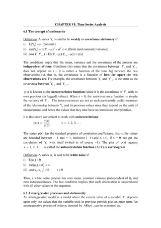
Figure 1(a) is a plot of a white noise process. The process has no trending behaviour,
and frequently crosses its mean value (zero), that is, it is stationary. A plot of a random
walk process is shown in Figure 1(b). We can see that the process has trends, that is, it
rises over time. This is a typical characteristic of non-stationary (unit-root) processes.
(a) A white noise process (b) A random walk process
Figure 1: Time series plot of white noise and random walk processes
6.4 Integrated processes and differencing
The difference operator  is defined as:
d d
t t
Y (1 Z) Y
   , d = 1, 2, 3, …
where Z is the lag operator: p
t t p
Z Y Y p 1, 2, 3, . . .

  .
e.g. First difference: 1
t t t t t t t 1
Y Y (1 Z)Y Y ZY Y Y
        
Second difference: 2 2 2
t t t
Y (1 Z) Y (1 2Z Z )Y
     
2
t t t t t 1 t 2
Y 2ZY Z Y Y 2Y Y
 
     
Consider the random walk process:
t t 1 t
Y Y u

 
where the error term t
u is white noise. We have seen that t
Y is a unit root process (that
is, that the root of the characteristic equation equals unity), and hence, is non-
stationary. The above equation can be written as:
t t 1 t 1 t 1 t
Y Y Y Y u
  
   
t t 1 t
Y Y u

  
t t
Y u
  
Since the error term t
u is white noise (which is stationary by definition), the first
difference t
Y
 is stationary. The series t
Y is said to be integrated of order one
(denoted by I(1)) since taking a first difference produces a stationary process.

5. 83 Applied Econometrics for Accounting and Finance
This concept can be generalized to consider the case where the series contains more
than one ‘unit root’. In such cases, the difference operator would need to be applied
more than once to induce stationarity. If a non-stationary series t
Y must be differenced
d times before it becomes stationary, then it is said to be integrated of order d. This
would be written as: t
Y ~ I(d) .
An I(0) series is a stationary series, while an I(1) series contains one unit root. An I(2)
series contains two unit roots and so would require differencing twice to induce
stationarity. The majority of financial and economic time series contain a single unit
root, although some are stationary and some have been argued to possibly contain two
unit roots.
6.5 Testing for a unit root
We need some kind of formal hypothesis testing procedure that answers the question,
‘given the sample data at hand, is it plausible that the true data generating process for Y
contains one or more unit roots?’ Consider the regression:
t t 1 t
Y Y u

     ……………… (2)
t t 1 t 1 t
Y Y ( 1)Y u
 
       
t t 1 t
y Y u

      
where 1
    . Note that if 1
  (or equivalently, if 0
  ), then Equation (2) is the
random walk process, and hence, non-stationary. The Dickey-Fuller (DF) test for a
unit root is carried out by testing the null hypothesis 0
H : 0
  (the series contains a
unit root) against the one-sided alternative 1
H : 0
  (the series is stationary). The test
statistic is:
ˆ
t
ˆ
se( )



where ̂ is the OLS estimator of  and ˆ
se( )
 is its standard error. Failing to reject the
null hypothesis means that there is a unit root.
In regressions involving trended data, Dickey and Fuller have shown that the
conventional test of significance (that is, the t-test) that compares the above test statistic
with the critical values from the standard t-table tends to incorrectly reject the null
hypothesis 0
H : 0
  . As a solution to this problem, they have derived an appropriate
set of critical values for testing the hypothesis that 0
H : 0
  . Thus, the critical values
for the above test are to be referred from such Dickey- Fuller tables.
The augmented Dickey-Fuller (ADF) test can accommodate higher order
autoregressive processes. For an AR(2) model ( t 1 t 1 2 t 2 t
Y Y Y u
 
    ), for instance,
the test is carried out in the context of the model:
t t 1 t 1 t
Y Y Y u
 
       
where 2
   and 1 2 1
     . The null hypothesis of a unit root is expressed as
0
H : 0
  (or 1 2 1
   ).

6. 84
CHAPTER VI: Time Series Analysis
Illustration: The following time plot is the export price of sesame in Ethiopia from
February 1998 to June 2013.
0
4,000
8,000
12,000
16,000
20,000
24,000
28,000
98 99 00 01 02 03 04 05 06 07 08 09 10 11 12 13
Export price of sesame
Figure 2: Time series plot of the export price of sesame in Ethiopia
We can see that the price of sesame exhibits an increasing trend over time. This might
be an indication that the process is non-stationary. To determine whether this is so, the
augmented Dickey-Fuller test is carried out. EViews output of the ADF test is shown
below:
Null Hypothesis: SESAME has a unit root
Exogenous: Constant, Linear Trend
Lag Length: 1 (Automatic - based on SIC, maxlag=13)
t-Statistic Prob.*
Augmented Dickey-Fuller test statistic 0.182840 0.9978
Test critical values: 1% level -4.008987
5% level -3.434569
10% level -3.141237
The ADF test statistic (0.182840) is greater than the critical values at 1%, 5% and 10%
significance levels (or the p-value (Prob.*) is greater than 10%). Thus, the null
hypothesis of a unit root cannot be rejected. This tells us that the export price of sesame
is a unit root process.
Since the series is non-stationary (has unit roots), we need to check if first differencing
removes the unit root problem. The result (EViews output) is shown below:
Null Hypothesis: D(SESAME) has a unit root
Exogenous: Constant, Linear Trend
Lag Length: 0 (Automatic - based on SIC, maxlag=13)
t-Statistic Prob.*
Augmented Dickey-Fuller test statistic -10.72704 0.0000
Test critical values: 1% level -4.008987
5% level -3.434569
10% level -3.141237
The p-value of the ADF test statistic for the first difference of the export price of
sesame is less than 0.01. Thus, we reject the null hypothesis and conclude that the first
differenced series is stationary, that is, the export price of sesame is integrated of order
one or I(1). Figure 3 is a time plot of the first difference of the export price of sesame.
We can observe that the series revolves around zero with no apparent trend.

7. 85 Applied Econometrics for Accounting and Finance
-1,200
-800
-400
0
400
800
1,200
98 99 00 01 02 03 04 05 06 07 08 09 10 11 12 13
D(SESAME)
Figure 3: Time series plot of the first difference of the export price of sesame
6.6 Non-stationarity and spurious regression
There are several reasons why the concept of stationarity is important and why it is
essential that variables that are non-stationary be treated differently from those that are
stationary. One of reasons is that the use of non-stationary data can lead to spurious
regressions.
If two stationary variables are generated as independent random series, when one of
those variables is regressed on the other, the t-ratio on the slope coefficient would be
expected not to be significantly different from zero, and the value of 2
R would be
expected to be very low. This seems obvious since the variables are not related to one
another. However, if two variables are trending over time, a regression of one on the
other could have a high 2
R even if the two are totally unrelated.
So, if standard regression techniques are applied to non-stationary series, the end result
could be a regression that ‘looks’ good under standard measures (significant coefficient
estimates and a high 2
R ), but which is really valueless or has no meaningful economic
interpretation. Such a model would be termed a ‘spurious regression’.
Illustration: The following EViews output pertains to a linear regression of the United
States (US) GDP on the total reserves of Ethiopia (including gold) from 1961 to 2008
(both in current USD). We can see that 2
R is large (73%) and the model is adequate as
judged by the F-test (p-value < 0.001). Moreover, the t-test indicates that the total
reserves of Ethiopia is significant at the 1% level, that is, total reserves of Ethiopia has
a significant influence on US GDP. But we know that the total reserves of Ethiopia (a
small economy) can never affect the US economy (as measured by US GDP). This is
clearly a spurious regression.
Dependent Variable: US_GDP
Method: Least Squares
Sample: 1961 2008
Variable Coefficient Std. Error t-Statistic Prob.
C 1.32E+12 4.81E+11 2.754921 0.0084
ETH_TOTAL_RESERVE 10383.57 924.2723 11.23432 0.0000
R-squared 0.732884
F-statistic 126.2099
Prob(F-statistic) 0.000000
The plots of two series are shown Figure 4 below. We can see that both have strongly
trending behaviour.

8. 86
CHAPTER VI: Time Series Analysis
Figure 4: Time plots of the total reserves of Ethiopia and US GDP
The augmented Dickey- Fuller test is carried out to determine whether the two series
are stationary or not. EViews output of the ADF tests is shown below. The p-values of
the ADF test statistics are both greater than 10%. Thus, both series are non-stationary.
Null Hypothesis: ETH_TOTAL_RESERVE has a unit root
Exogenous: Constant, Linear Trend
Lag Length: 0 (Automatic - based on SIC, maxlag=9)
t-Statistic Prob.*
Augmented Dickey-Fuller test statistic -3.118509 0.1140
Test critical values: 1% level -4.165756
5% level -3.508508
10% level -3.184230
Null Hypothesis: US_GDP has a unit root
Exogenous: Constant, Linear Trend
Lag Length: 3 (Automatic - based on SIC, maxlag=9)
t-Statistic Prob.*
Augmented Dickey-Fuller test statistic 0.531672 0.9991
Test critical values: 1% level -4.180911
5% level -3.515523
10% level -3.188259
The ADF tests on first differences of the two series (shown below) reveal that both
series are integrated of order one.
Null Hypothesis: D(ETH_TOTAL_RESERVE) has a unit root
Lag Length: 3 (Automatic - based on SIC, maxlag=9)
t-Statistic Prob.*
Augmented Dickey-Fuller test statistic -5.805088 0.0001
Test critical values: 1% level -4.186481
5% level -3.518090
10% level -3.189732
Null Hypothesis: D(US_GDP) has a unit root
Lag Length: 2 (Automatic - based on SIC, maxlag=9)
t-Statistic Prob.*
Augmented Dickey-Fuller test statistic -5.292081 0.0004
Test critical values: 1% level -4.180911
5% level -3.515523
10% level -3.188259
Total reserves (current USD)
0
200000000
400000000
600000000
800000000
1000000000
1200000000
1400000000
1600000000
1800000000
2000000000
1961
1963
1965
1967
1969
1971
1973
1975
1977
1979
1981
1983
1985
1987
1989
1991
1993
1995
1997
1999
2001
2003
2005
2007
2009
US GDP (current USD)
0
2000000000000
4000000000000
6000000000000
8000000000000
10000000000000
12000000000000
14000000000000
16000000000000
1961
1963
1965
1967
1969
1971
1973
1975
1977
1979
1981
1983
1985
1987
1989
1991
1993
1995
1997
1999
2001
2003
2005
2007

9. 87 Applied Econometrics for Accounting and Finance
The results of a linear regression of the first difference of US GDP on the first
difference of total reserves of Ethiopia are shown below. Note that this is not
spurious regression since the differenced series are both stationary. We can see that the
value of 2
R is zero and the F-statistic is insignificant (p-value = 0.999 > 0.05). Thus,
there is no relationship between US GDP and the total reserves of Ethiopia. The
implication is that the significant relationship that we obtained earlier was simply a
consequence of the underlying trend in both series.
Dependent Variable: D(US_GDP)
Method: Least Squares
Sample (adjusted): 1962 2008
Variable Coefficient Std. Error t-Statistic Prob.
C 3.01E+11 3.06E+10 9.854698 0.0000
D(ETH_TOTAL_RESERVE) -0.188617 171.1093 -0.001102 0.9991
R-squared 0.000000
F-statistic 1.22E-06
Prob(F-statistic) 0.999125