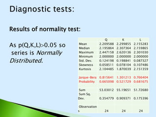
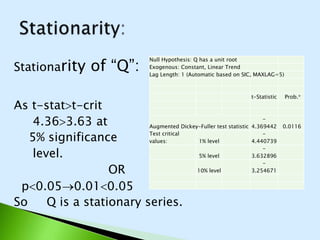
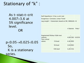
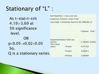
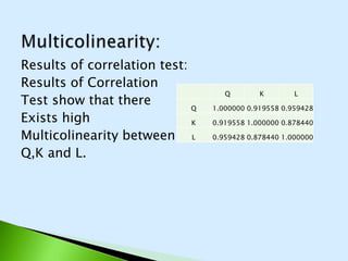
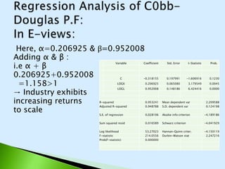
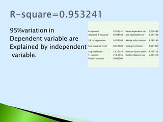
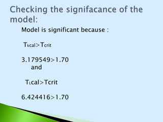
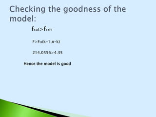
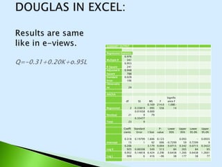
Cobb-douglas production 
function 
Sub Topics 
Background: 
Definition: 
Equation: 
Diagnostic Tests: 
Estimation of parameters in regression:
Background: 
Developed by Paul 
Douglas and C. W. 
Cobb in the 1930’s.
Definition: 
Cobb Douglas is a 
Mathematical Formula that 
relates Labor Capital and Output. 
Cobb- Douglas equation: 
Q=AKaLb
Cobb-douglas data file 
Q K L 
100 100 100 
101 100 105 
112 107 110 
122 114 118 
124 122 123 
122 131 116 
143 138 125 
152 149 133 
151 163 138 
126 176 121 
155 185 140 
159 198 144 
153 208 145 
177 216 152 
184 226 154 
169 236 149 
189 244 154 
225 266 182 
227 298 196 
223 335 200 
280 366 193 
231 387 193 
179 407 147 
240 417 161
Log transformation for 
regression Log Q Log K Log L 
Following Formula is Used for 
Log Transformation 
=(log(A)) so on…. 
2 2 2 
2.0043 
21 2 
2.0211 
89 
2.0492 
18 
2.0293 
84 
2.0413 
93 
2.0863 
6 
2.0569 
05 
2.0718 
82 
2.0934 
22 
2.0863 
6 
2.0899 
05 
2.0863 
6 
2.1172 
71 
2.0644 
58 
2.1553 
36 
2.1398 
79 
2.0969 
1 
2.1818 
44 
2.1731 
86 
2.1238 
52 
2.1789 
77 
2.2121 
88 
2.1398 
79 
2.1003 
71 
2.2455 
13 
2.0827 
85 
2.1903 
32 
2.2671 
72 
2.1461 
28 
2.2013 
97 
2.2966 
65 
2.1583 
62 
2.1846 
91 
2.3180 
63 
2.1613 
68 
2.2479 
73 
2.3344 
54 
2.1818 
44 
2.2648 
18 
2.3541 
08 
2.1875 
21 
2.2278 
87 
2.3729 
12 
2.1731 
86 
2.2764 
62 
2.3873 
9 
2.1875 
21 
2.3521 
83 
2.4248 
82 
2.2600 
71
Diagnostic tests: 
Results of normality test: 
As p(Q,K,L)>0.05 so 
series is Normally 
Distributed. 
Q K L 
Mean 2.209588 2.299855 2.155283 
Median 2.195864 2.307364 2.159865 
Maximum 2.447158 2.620136 2.301030 
Minimum 2.000000 2.000000 2.000000 
Std. Dev. 0.124198 0.198841 0.087327 
Skewness 0.058511 0.078104 0.107486 
Kurtosis 2.104485 1.870039 2.151359 
Jarque-Bera 0.815641 1.301213 0.766404 
Probability 0.665098 0.521729 0.681675 
Sum 53.03012 55.19651 51.72680 
Sum Sq. 
Dev. 0.354779 0.909371 0.175396 
Observations 24 24 24
Stationarity: 
Stationarity of “Q”: 
As t-stat>t-crit 
4.36>3.63 at 
5% significance 
level. 
OR 
Null Hypothesis: Q has a unit root 
Exogenous: Constant, Linear Trend 
Lag Length: 1 (Automatic based on SIC, MAXLAG=5) 
p<0.05®0.01<0.05 
So Q is a stationary series. 
t-Statistic Prob.* 
Augmented Dickey-Fuller test statistic -4.369442 0.0116 
Test critical values: 1% level -4.440739 
5% level -3.632896 
10% level -3.254671
Null Hypothesis: K has a unit root 
Exogenous: Constant, Linear Trend 
Lag Length: 1 (Automatic based on SIC, MAXLAG=4) 
t-Statistic Prob.* 
Augmented Dickey-Fuller test statistic -4.007282 0.0250 
Test critical values: 1% level -4.467895 
5% level -3.644963 
10% level -3.261452 
Stationary of “k” : 
As t-stat>t-crit 
4.007>3.6 at 
5% significance 
level. 
OR 
p<0.05®0.025<0.05 
So, 
K is a stationary 
series.
9 
Stationary of “L” : 
As t-stat>t-crit 
4.19>3.69 at 
5% significance 
level. 
OR 
p<0.05®0.02<0.05 
So, 
Q is a stationary series. 
Null Hypothesis: L has a unit root 
Exogenous: Constant, Linear Trend 
Lag Length: 4 (Automatic based on SIC, MAXLAG=4) 
t-Statistic Prob.* 
Augmented Dickey-Fuller test statistic -4.196949 0.0200 
Test critical 
values: 1% level -4.571559 
5% level -3.690814 
10% level -3.286909
Multicolinearity: 
Results of correlation test: 
Results of Correlation 
Test show that there 
Exists high 
Multicolinearity between 
Q,K and L. 
Q K L 
Q 1.000000 0.919558 0.959428 
K 0.919558 1.000000 0.878440 
L 0.959428 0.878440 1.000000
Regression Analysis of C0bb- 
Douglas P.F: 
In E-views: 
 
Here, α=0.206925 & 
Adding α & β : 
i.e α + β 
0.206925+0.952008 
=1.158>1 
→ Industry exhibits 
increasing returns 
to scale 
Variable Coefficient Std. Error t-Statistic Prob. 
C -0.318155 0.197991 -1.606916 0.1230 
LOGK 0.206925 0.065080 3.179549 0.0045 
LOGL 0.952008 0.148186 6.424416 0.0000 
R-squared 0.953241 Mean dependent var 2.209588 
Adjusted R-squared 0.948788 S.D. dependent var 0.124198 
S.E. of regression 0.028106 Akaike info criterion -4.189186 
Sum squared resid 0.016589 Schwarz criterion -4.041929 
Log likelihood 53.27023 Hannan-Quinn criter. -4.150119 
F-statistic 214.0556 Durbin-Watson stat 2.247216 
Prob(F-statistic) 0.000000
Interpretation of r-square: 
 R-squared is a statistical measure. It is also known as the 
coefficient of determination, or the coefficient of multiple 
determination for multiple regression. 
 It is the percentage of the response variable variation that is 
explained by a linear model. 
 → R-squared = Explained variation / Total variation 
 R-squared is always between 0 and 100%: 
 0% indicates that the model explains none of the variability 
of the response data around its mean. 
 100% indicates that the model explains all the variability of 
the response data around its mean.
R-square=0.953241 
95%variation in 
Dependent variable are 
Explained by independent 
variable. 
R-squared 0.953241 Mean dependent var 2.209588 
Adjusted R-squared 0.948788 S.D. dependent var 0.124198 
S.E. of regression 0.028106 Akaike info criterion -4.189186 
Sum squared resid 0.016589 Schwarz criterion -4.041929 
Log likelihood 53.27023 Hannan-Quinn criter. -4.150119 
F-statistic 214.0556 Durbin-Watson stat 2.247216 
Prob(F-statistic) 0.000000
Checking the signifacance of the 
model: 
Model is significant because : 
Tkcal>Tcrit 
3.179549>1.70 
and 
TLcal>Tcrit 
6.424416>1.70
Checking the goodness of the 
model: 
fcal>fcrit 
F>Fa(k-1,n-k) 
214.0556>4.35 
Hence the model is good
SUMMARY 
OUTPUT 
Regression 
Statistics 
Multiple R 
0.9763 
41 
R Square 
0.9532 
41 
Adjusted 
R Square 
0.9487 
88 
Standard 
Error 
0.0281 
06 
Observati 
ons 24 
ANOVA 
df SS MS F 
Significa 
nce F 
Regressio 
n 2 0.33819 
0.169 
095 
214.0 
556 
1.08E- 
14 
Residual 21 0.016589 
0.000 
79 
Total 23 0.354779 
Coeffic 
ients 
Standard 
Error t Stat 
P-value 
Lower 
95% 
Upper 
95% 
Lower 
95.0% 
Upper 
95.0% 
Intercept 
- 
0.3181 
5 0.197991 
- 
1.606 
92 
0.123 
006 -0.7299 
0.0935 
9 -0.7299 0.09359 
Log K 
0.2069 
25 0.06508 
3.179 
549 
0.004 
513 
0.07158 
4 
0.3422 
65 
0.07158 
4 
0.34226 
5 
Log L 
0.9520 
08 0.148186 
6.424 
416 
2.29E 
-06 
0.64383 
8 
1.2601 
77 
0.64383 
8 
1.26017 
7 
REGRESSION ANALYSIS OF 
COBB-DOUGLAS IN EXCEL: 
Results are same 
like in e-views. 
Q=-0.31+0.20K+o.95L
The End…. ☺

Cobb-douglas production function

  • 1.
    Cobb-douglas production function Sub Topics Background: Definition: Equation: Diagnostic Tests: Estimation of parameters in regression:
  • 2.
    Background: Developed byPaul Douglas and C. W. Cobb in the 1930’s.
  • 3.
    Definition: Cobb Douglasis a Mathematical Formula that relates Labor Capital and Output. Cobb- Douglas equation: Q=AKaLb
  • 4.
    Cobb-douglas data file Q K L 100 100 100 101 100 105 112 107 110 122 114 118 124 122 123 122 131 116 143 138 125 152 149 133 151 163 138 126 176 121 155 185 140 159 198 144 153 208 145 177 216 152 184 226 154 169 236 149 189 244 154 225 266 182 227 298 196 223 335 200 280 366 193 231 387 193 179 407 147 240 417 161
  • 5.
    Log transformation for regression Log Q Log K Log L Following Formula is Used for Log Transformation =(log(A)) so on…. 2 2 2 2.0043 21 2 2.0211 89 2.0492 18 2.0293 84 2.0413 93 2.0863 6 2.0569 05 2.0718 82 2.0934 22 2.0863 6 2.0899 05 2.0863 6 2.1172 71 2.0644 58 2.1553 36 2.1398 79 2.0969 1 2.1818 44 2.1731 86 2.1238 52 2.1789 77 2.2121 88 2.1398 79 2.1003 71 2.2455 13 2.0827 85 2.1903 32 2.2671 72 2.1461 28 2.2013 97 2.2966 65 2.1583 62 2.1846 91 2.3180 63 2.1613 68 2.2479 73 2.3344 54 2.1818 44 2.2648 18 2.3541 08 2.1875 21 2.2278 87 2.3729 12 2.1731 86 2.2764 62 2.3873 9 2.1875 21 2.3521 83 2.4248 82 2.2600 71
  • 6.
    Diagnostic tests: Resultsof normality test: As p(Q,K,L)>0.05 so series is Normally Distributed. Q K L Mean 2.209588 2.299855 2.155283 Median 2.195864 2.307364 2.159865 Maximum 2.447158 2.620136 2.301030 Minimum 2.000000 2.000000 2.000000 Std. Dev. 0.124198 0.198841 0.087327 Skewness 0.058511 0.078104 0.107486 Kurtosis 2.104485 1.870039 2.151359 Jarque-Bera 0.815641 1.301213 0.766404 Probability 0.665098 0.521729 0.681675 Sum 53.03012 55.19651 51.72680 Sum Sq. Dev. 0.354779 0.909371 0.175396 Observations 24 24 24
  • 7.
    Stationarity: Stationarity of“Q”: As t-stat>t-crit 4.36>3.63 at 5% significance level. OR Null Hypothesis: Q has a unit root Exogenous: Constant, Linear Trend Lag Length: 1 (Automatic based on SIC, MAXLAG=5) p<0.05®0.01<0.05 So Q is a stationary series. t-Statistic Prob.* Augmented Dickey-Fuller test statistic -4.369442 0.0116 Test critical values: 1% level -4.440739 5% level -3.632896 10% level -3.254671
  • 8.
    Null Hypothesis: Khas a unit root Exogenous: Constant, Linear Trend Lag Length: 1 (Automatic based on SIC, MAXLAG=4) t-Statistic Prob.* Augmented Dickey-Fuller test statistic -4.007282 0.0250 Test critical values: 1% level -4.467895 5% level -3.644963 10% level -3.261452 Stationary of “k” : As t-stat>t-crit 4.007>3.6 at 5% significance level. OR p<0.05®0.025<0.05 So, K is a stationary series.
  • 9.
    9 Stationary of“L” : As t-stat>t-crit 4.19>3.69 at 5% significance level. OR p<0.05®0.02<0.05 So, Q is a stationary series. Null Hypothesis: L has a unit root Exogenous: Constant, Linear Trend Lag Length: 4 (Automatic based on SIC, MAXLAG=4) t-Statistic Prob.* Augmented Dickey-Fuller test statistic -4.196949 0.0200 Test critical values: 1% level -4.571559 5% level -3.690814 10% level -3.286909
  • 10.
    Multicolinearity: Results ofcorrelation test: Results of Correlation Test show that there Exists high Multicolinearity between Q,K and L. Q K L Q 1.000000 0.919558 0.959428 K 0.919558 1.000000 0.878440 L 0.959428 0.878440 1.000000
  • 11.
    Regression Analysis ofC0bb- Douglas P.F: In E-views:  Here, α=0.206925 & Adding α & β : i.e α + β 0.206925+0.952008 =1.158>1 → Industry exhibits increasing returns to scale Variable Coefficient Std. Error t-Statistic Prob. C -0.318155 0.197991 -1.606916 0.1230 LOGK 0.206925 0.065080 3.179549 0.0045 LOGL 0.952008 0.148186 6.424416 0.0000 R-squared 0.953241 Mean dependent var 2.209588 Adjusted R-squared 0.948788 S.D. dependent var 0.124198 S.E. of regression 0.028106 Akaike info criterion -4.189186 Sum squared resid 0.016589 Schwarz criterion -4.041929 Log likelihood 53.27023 Hannan-Quinn criter. -4.150119 F-statistic 214.0556 Durbin-Watson stat 2.247216 Prob(F-statistic) 0.000000
  • 12.
    Interpretation of r-square:  R-squared is a statistical measure. It is also known as the coefficient of determination, or the coefficient of multiple determination for multiple regression.  It is the percentage of the response variable variation that is explained by a linear model.  → R-squared = Explained variation / Total variation  R-squared is always between 0 and 100%:  0% indicates that the model explains none of the variability of the response data around its mean.  100% indicates that the model explains all the variability of the response data around its mean.
  • 13.
    R-square=0.953241 95%variation in Dependent variable are Explained by independent variable. R-squared 0.953241 Mean dependent var 2.209588 Adjusted R-squared 0.948788 S.D. dependent var 0.124198 S.E. of regression 0.028106 Akaike info criterion -4.189186 Sum squared resid 0.016589 Schwarz criterion -4.041929 Log likelihood 53.27023 Hannan-Quinn criter. -4.150119 F-statistic 214.0556 Durbin-Watson stat 2.247216 Prob(F-statistic) 0.000000
  • 14.
    Checking the signifacanceof the model: Model is significant because : Tkcal>Tcrit 3.179549>1.70 and TLcal>Tcrit 6.424416>1.70
  • 15.
    Checking the goodnessof the model: fcal>fcrit F>Fa(k-1,n-k) 214.0556>4.35 Hence the model is good
  • 16.
    SUMMARY OUTPUT Regression Statistics Multiple R 0.9763 41 R Square 0.9532 41 Adjusted R Square 0.9487 88 Standard Error 0.0281 06 Observati ons 24 ANOVA df SS MS F Significa nce F Regressio n 2 0.33819 0.169 095 214.0 556 1.08E- 14 Residual 21 0.016589 0.000 79 Total 23 0.354779 Coeffic ients Standard Error t Stat P-value Lower 95% Upper 95% Lower 95.0% Upper 95.0% Intercept - 0.3181 5 0.197991 - 1.606 92 0.123 006 -0.7299 0.0935 9 -0.7299 0.09359 Log K 0.2069 25 0.06508 3.179 549 0.004 513 0.07158 4 0.3422 65 0.07158 4 0.34226 5 Log L 0.9520 08 0.148186 6.424 416 2.29E -06 0.64383 8 1.2601 77 0.64383 8 1.26017 7 REGRESSION ANALYSIS OF COBB-DOUGLAS IN EXCEL: Results are same like in e-views. Q=-0.31+0.20K+o.95L
  • 17.