The document discusses the topic of autocorrelation. It begins by defining autocorrelation as data that is correlated with itself over successive time periods, rather than being correlated with other external data. It then explains the concept of autocorrelation and how it violates the classical linear regression assumption that disturbances are independent over time. Several potential sources of autocorrelation are described, including omitted variables, interpolation of data, and misspecification of the random error term. The document concludes by providing mathematical expressions that describe how the mean, variance, and covariance of autocorrelated disturbances differ from the independent case.

1. ACADEMIC WRITING
Name : ADITHYA T DAS
Reg no : 3a2dc31eede711e9a75699c83cf6ce8e
Department of Mathematics and Statistics
Central University of Punjab Bathinda
TOPIC : AUTOCORRELATION

2. ACKNOWLEDGEMENT
 I would like to express my gratitude to SWAYAM who offered me the
course ACADEMIC WRITING and also I am thankful to Prof. Ajay Semalty.
Who take classes on this topic.

3. What is Autocorrelation :
 The auto part of autocorrelation is from the Greek word for self, and
autocorrelation means data that is correlated with itself, as opposed to
being correlated with some other data.
 Autocorrelation means the data correlated with itself.
 Autocorrelation can also be referred to as lagged correlation or serial
correlation

4. Concept of autocorrelation:
 One of the classical linear regression model (CLRM)
assumption is that, the disturbance term related to any other
observation is not influenced by the disturbance term to any
other observation E(ui,uj) = 0 , i ≠ j
If this assumption is Not satisfied that is if the value of u
in any particular period of time is correlated with its own
preceding value.

5.  Disturbance are not pairwise independent but pairwise
autocorrelated.
 Which mostly occur in time series data.

6. Definition :
One period of time has great effect on another period of time .
So disturbance term in two different period of time is closely
related with each other.
that is,
E ( ui , uj ) ≠ 0 .

7. Sources of Autocorrelation
Omitted explanatory variables :
 Most of economics variables tends to be auto correlated. If
an auto correlated variables has been excluded from the
model its influence will be reflected in disturbance term
whose valus will be correlated this may be called quasi auto
correlated.
 It is due to omission of auto correlation variable.

8. Interpolation in the statistical observation :
 Most of time series data involve interpolation and
smoothing process which do average the true disturbance
term over the successive time periods so successive value of
ui are interrelated.

9. Misspecification of true random term ui :
 It may be expected that successive value of ui are
correlated. Random factors such as wars, drought, strikes has
great influence over a long period of time.
e.g. ; low agriculture cropping in one period of time
has influence on several other variables other period of time.

10. The first order autocorrelation :
 The simplest and most commonly observed is the first order
autocorrelation
 Autoregressive structure is : ut = ρ ut-1 + vt
 ρ is called the first order autocorrelation coefficient
 values between -1 to +1
 ρ is zero then there is no autocorrelation
 ρ is 1 then there is positive autocorrelation
 ρ is -1 then there is negative autocorrelation.

12. Mean of autocorrelated u’s :
ut=Σ ρr vt-r is the value of error term when it is autocorrelated
with a first order autoregressive scheme.
E(ut) = E Σ ρr vt-r
= Σ ρr E (vt-r )
by the assumption of distribution of v we have,
E (vt-r ) = 0
therefore E (ut ) = 0 ( t = 1,2,3,…,n)

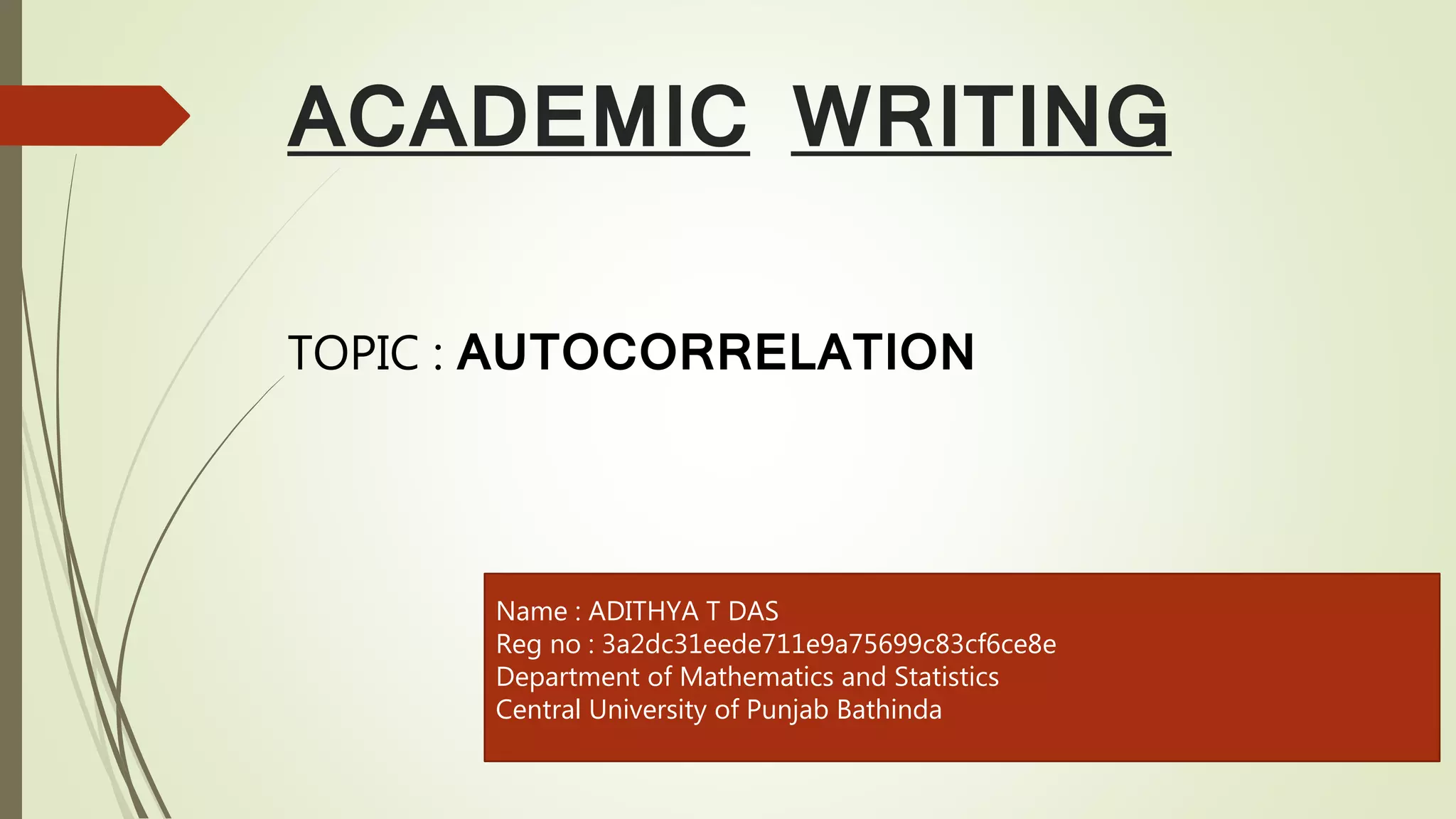
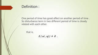
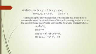
13. Variance of the autocorrelated u’s :
By the definition of the variance we have
E(ut
2) = E [ Σ ρr vt-r ] 2
= Σ (ρr )2 E( vt-r ) 2
= Σ (ρr )2 var( vt-r)
= Σ ρ2r σ2
v
= σ2
v ( 1+ ρ2 + ρ4 + ρ6 + … )
E(ut
2) = σ2
v [ 1/ 1- ρ2 ]
Or var( ut) = σ2
v / (1- ρ2 )

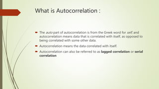
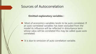
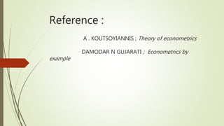
14. Covariance of the autocorrelated u’s :
given that ut = vt + ρ vt-2 + ρ2 vt-2 + . . .
and ut-1 = vt-1+ ρ vt-2 + ρ2 vt-3 + . . .
we obtain
cov(ut ut-1) = E {[ut –E(ut)] [ut-1 – E(ut-1)]} = E [ut ut-1]
= E [(vt + ρ vt-1 + ρ2 vt-2 +…)(vt-1 + ρ vt-2 + ρ2 vt-3 +…)]
= E[{vt + ρ (vt-1 + ρ vt-2 +…)}(vt-1 + ρ vt-2 + ρ2 vt-3 +…)]
= E [(vt )( vt-1 + ρ vt-2 + ρ2 vt-3 +…)]+E[ ρ (vt-1 + ρ vt-2 +…)2]
= 0 + ρ E(vt-1 + ρ vt-2 +…)2
= ρ E(v2
t-1 + ρ2 v2
t-2 +…+ cross product)
= ρ(σ2
v + ρ2σ2
v + …+ 0)
= ρ[σ2
v (1+ ρ2+ ρ4 + ρ6+…)] = ρσ2
v ( 1/ 1- ρ2) ( for |ρ| ˂ 1)
= ρσ2
v
cont…

15. similarly , cov (ut ut-2 ) = E (ut ut-2 )= ρ2σ2
u
cov (ut ut-s ) = ρs σ2
u (for s ≠ t )
summarising the above discussion we conclude that when there is
autocorrelation of the simple form of first order autoregressive scheme,
the autocorrelated disturbance term has the following characteristics ,
ut=Σ ρr vt-r
E(ut) = 0
var( ut) = σ2
v / (1- ρ2 ) = σ2
u
cov (ut ut-s ) = ρs σ2
u ≠ 0

16. Reference :
A . KOUTSOYIANNIS ; Theory of econometrics
DAMODAR N GUJARATI ; Econometrics by
example

17. Feedback :
The course ACADEMIC WRITING offered by SWAYAM is a good program for students
who are studying post graduation and PhD Scholars as well. By doing this course we
got an idea about what is academic writing is , also about plagiarism and what is
research paper , how to done it etc. By doing this course students got a brief idea
about these topics and this is really good course, Which helps all the students.