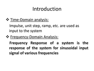
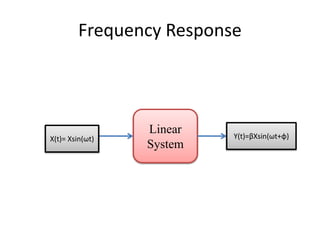
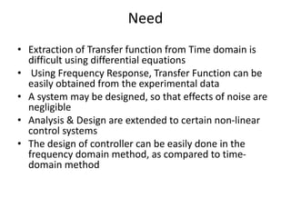
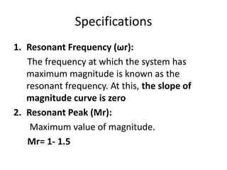
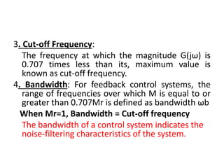
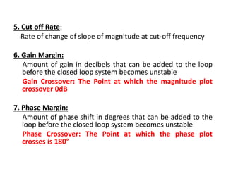
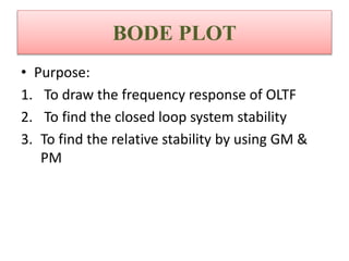
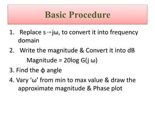
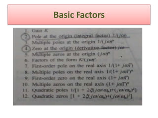
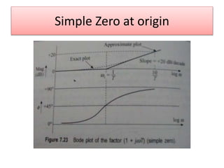
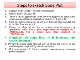
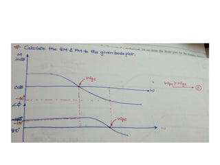
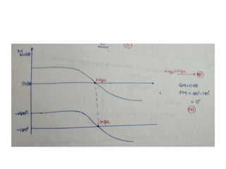
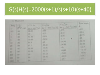
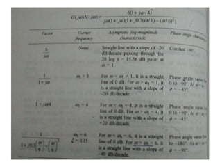
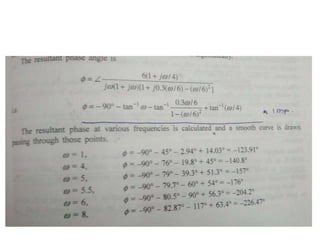
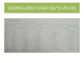
This document discusses frequency domain analysis and creating Bode plots. Frequency domain analysis examines a system's frequency response by using sinusoidal inputs rather than impulse inputs used in time domain analysis. A Bode plot graphs the magnitude and phase of a system's frequency response on logarithmic and linear scales. It can be used to determine stability margins like gain margin and phase margin. The document provides steps for sketching a Bode plot from a transfer function including identifying poles, zeros and gain. Key aspects of a Bode plot like bandwidth, resonant frequency and cut-off frequency are also defined. Examples of Bode plots for two transfer functions are included.

1. Unit 5
Frequency domain Analysis
Prajakta J Pardeshi
MITCOE
Pune

2. Introduction
 Time-Domain analysis:
Impulse, unit step, ramp, etc. are used as
input to the system
 Frequency-Domain Analysis:
Frequency Response of a system is the
response of the system for sinusoidal input
signal of various frequencies

3. Frequency Response
Linear
System
X(t)= Xsin(ωt) Y(t)=βXsin(ωt+φ)

4. Need
• Extraction of Transfer function from Time domain is
difficult using differential equations
• Using Frequency Response, Transfer Function can be
easily obtained from the experimental data
• A system may be designed, so that effects of noise are
negligible
• Analysis & Design are extended to certain non-linear
control systems
• The design of controller can be easily done in the
frequency domain method, as compared to time-
domain method

5. Specifications
1. Resonant Frequency (ωr):
The frequency at which the system has
maximum magnitude is known as the
resonant frequency. At this, the slope of
magnitude curve is zero
2. Resonant Peak (Mr):
Maximum value of magnitude.
Mr= 1- 1.5

6. 3. Cut-off Frequency:
The frequency at which the magnitude G(jω) is
0.707 times less than its, maximum value is
known as cut-off frequency.
4. Bandwidth: For feedback control systems, the
range of frequencies over which M is equal to or
greater than 0.707Mr is defined as bandwidth ωb
When Mr=1, Bandwidth = Cut-off frequency
The bandwidth of a control system indicates the
noise-filtering characteristics of the system.

7. 5. Cut off Rate:
Rate of change of slope of magnitude at cut-off frequency
6. Gain Margin:
Amount of gain in decibels that can be added to the loop
before the closed loop system becomes unstable
Gain Crossover: The Point at which the magnitude plot
crossover 0dB
7. Phase Margin:
Amount of phase shift in degrees that can be added to the
loop before the closed loop system becomes unstable
Phase Crossover: The Point at which the phase plot
crosses is 180°

8. BODE PLOT
• Purpose:
1. To draw the frequency response of OLTF
2. To find the closed loop system stability
3. To find the relative stability by using GM &
PM

9. • The Bode Plot consists of two parts:
1. Magnitude Plot
2. Phase Plot
BODE PLOT

10. Semilog paper

11. Basic Procedure
1. Replace s jω, to convert it into frequency
domain
2. Write the magnitude & Convert it into dB
Magnitude = 20log G(j ω)
3. Find the φ angle
4. Vary ‘ω’ from min to max value & draw the
approximate magnitude & Phase plot

12. Basic Factors

13. Constant Gain K (Shift K)

14. Pole at Origin

15. Zero at Origin

16. Simple pole at origin

17. Simple Zero at origin

18. Comparison

19. Comparison

20. 1. Express given G(s)H(s) in time constant form
2. Draw a line of 20LogK dB
3. Draw a line of appropriate slope representing poles or zeros at the
origin, passing through intersection point of ω=1 and 0 dB
4. Shift this intersection point on 20LogK line and draw parallel line
to the line drawn in step 3
5. Change the slope of this line at various corner frequencies by
appropriate value. For a pole, slope must be changed by -
20dB/Decade, For a simple zero slope changed by
+20dB/Decade .
• Continue this slope line, till it intersects last
corner frequency
6. Prepare the phase angle plot and table & obtain the table of ω and
resultant phase angle φR by actual calculation.
7. Plot these points , & Draw a smooth curve obtaining necessary
phase angle plot
Steps to sketch Bode Plot

21. Gain & Phase
Gain Margin
• Factor by which system gain
is increased to bring the
system to the verge of
stability
• Gain crossover: ωgc
• The frequency at which the
magnitude=1 in linear and
0 in dB.
Phase Margin
• Additional phase lag
required to ass system at
ωgc to bring system to
stability
• Phase cross over : ωpc
• The frequency at which
angle is -180 degre

23. • Gain Margin
• The gain margin (GM) is the factor by which the gain is less than the
neutral stability value. We can usually read the gain margin directly from
the bode plot. This is done by calculating the vertical distance between
the curve and the at the frequency.
• Phase Margin
• Another quantity related to determining stability margin is the phase
margin (PM). This is a different way to measure how well stability
conditions are met in a given system. Phase margin is determined by how
much the phase of exceeds.
• The above figure shows that, for a system to be stable, a positive PM is
required. From the figures, we can also see that the GM indicates the
amount that the gain can increase before a system becomes unstable.
The PM is calculated by measuring the difference between the and when
crosses the circle . The stable case receives the phase margin’s positive
value.

24. Crossover Frequency
• A gain of factor 1 (equivalent to 0 dB) where both input
and output are at the same voltage level and
impedance is known as unity gain. When the gain is at
this frequency, it is often referred to as crossover
frequency.
• Frequency-response design is practical because we can
easily evaluate how gain changes affect certain aspects
of systems. With frequency-response design, we can
determine the phase margin for any value of without
needing to redraw the magnitude or phase
information. All we have to do is indicate where for
certain trial values of

27. G(s)H(s)=2000(s+1)/s(s+10)(s+40)

30. G(s)H(s)=20(s+1)/s(s+5)(s^2+2S+10)