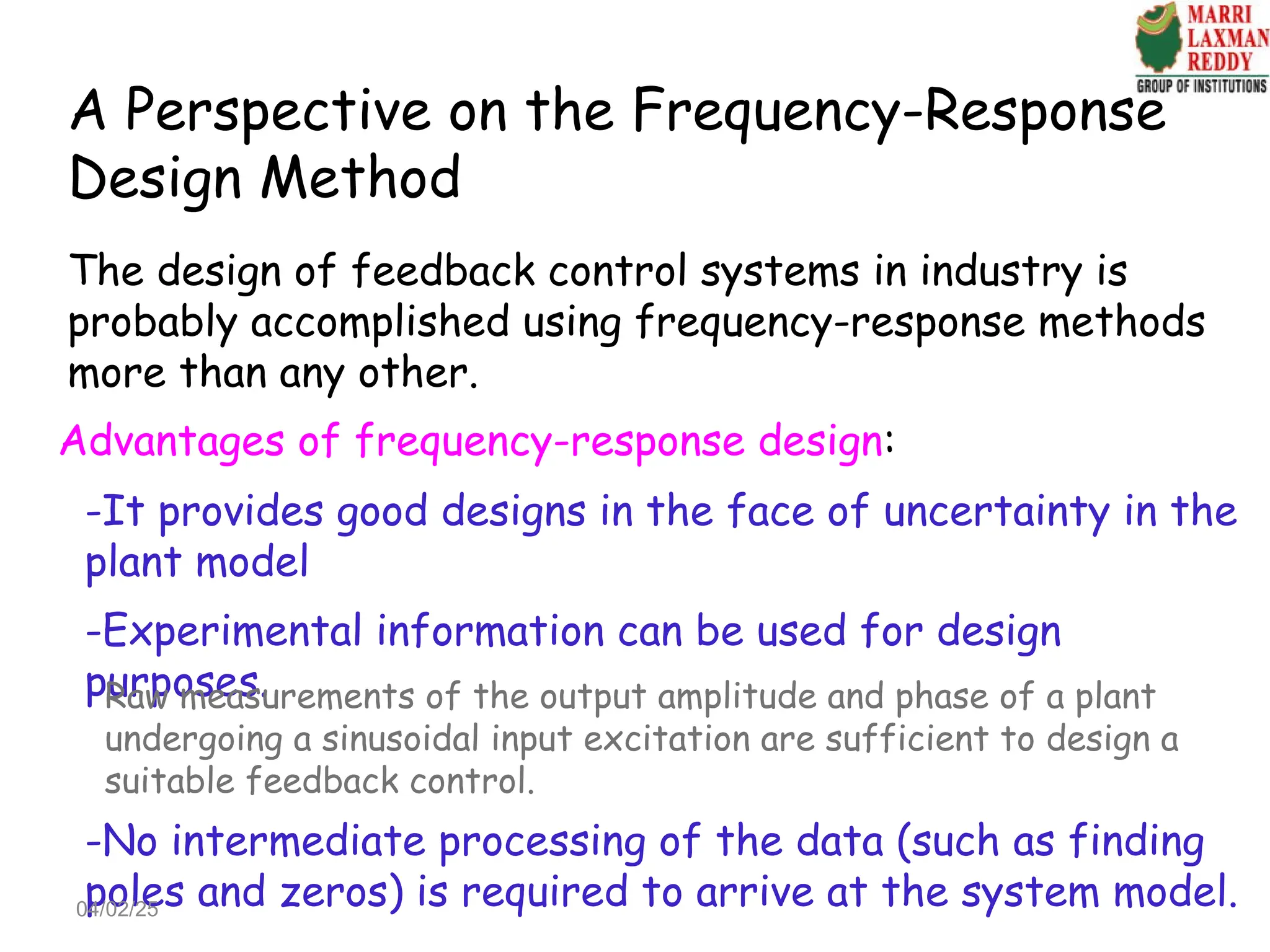
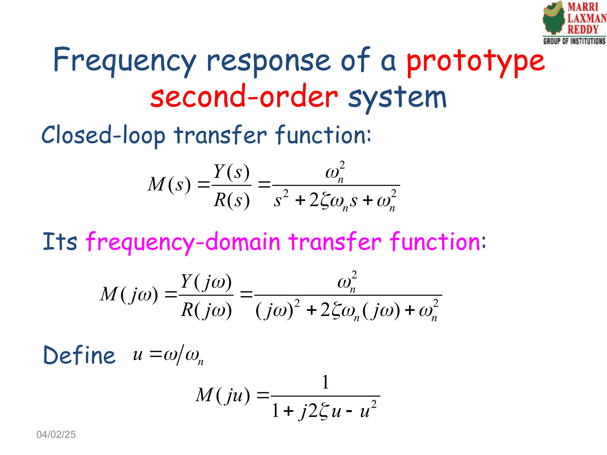
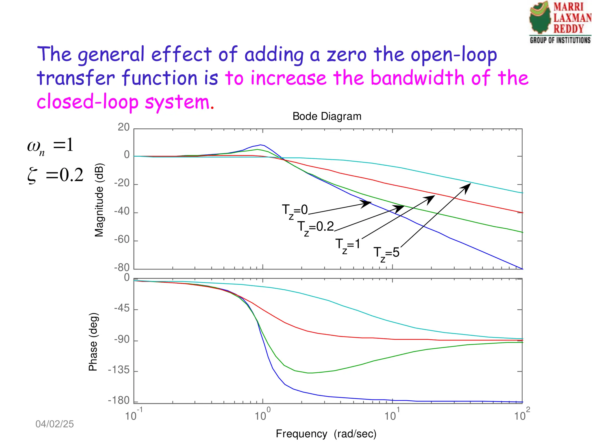
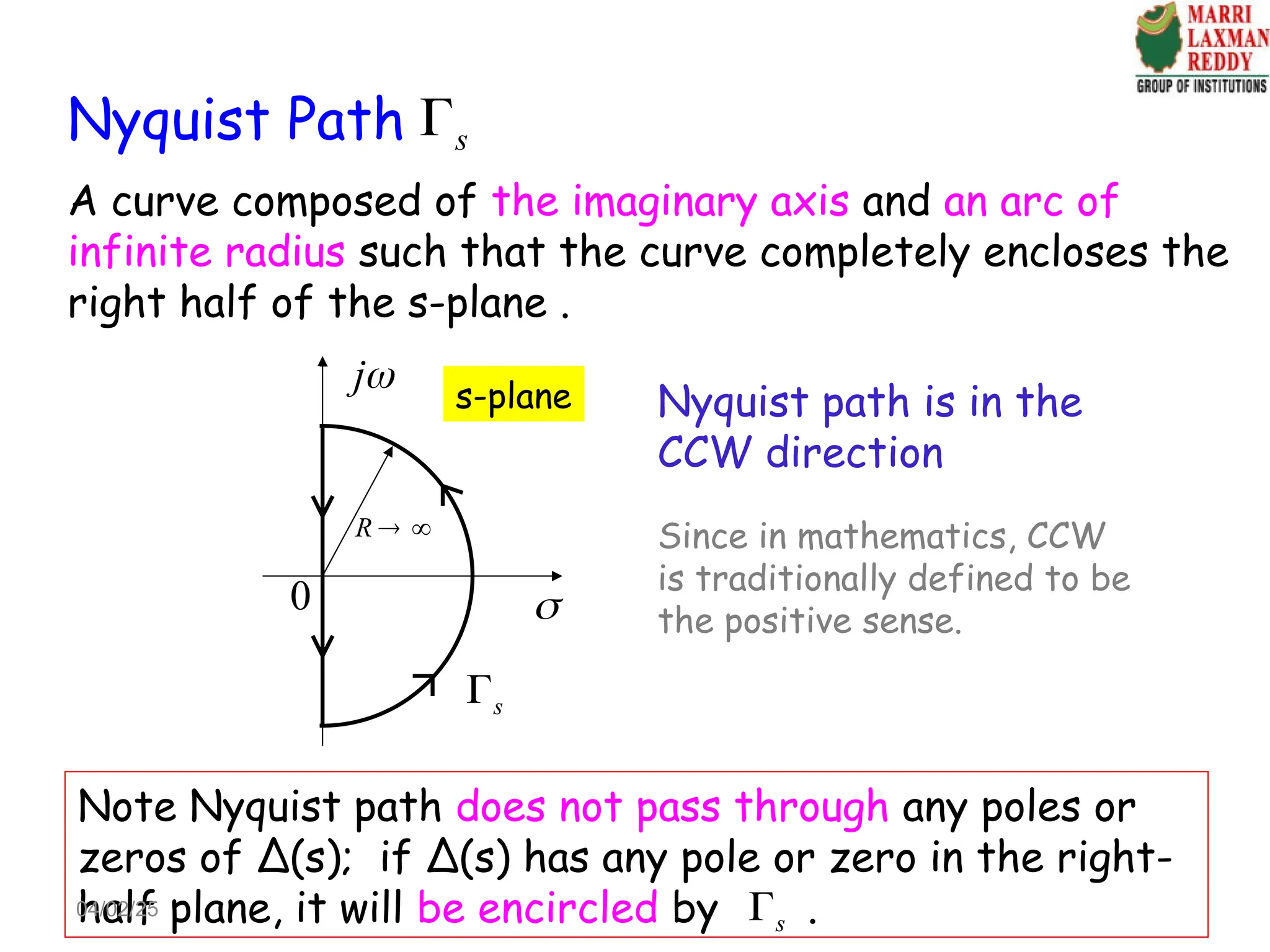
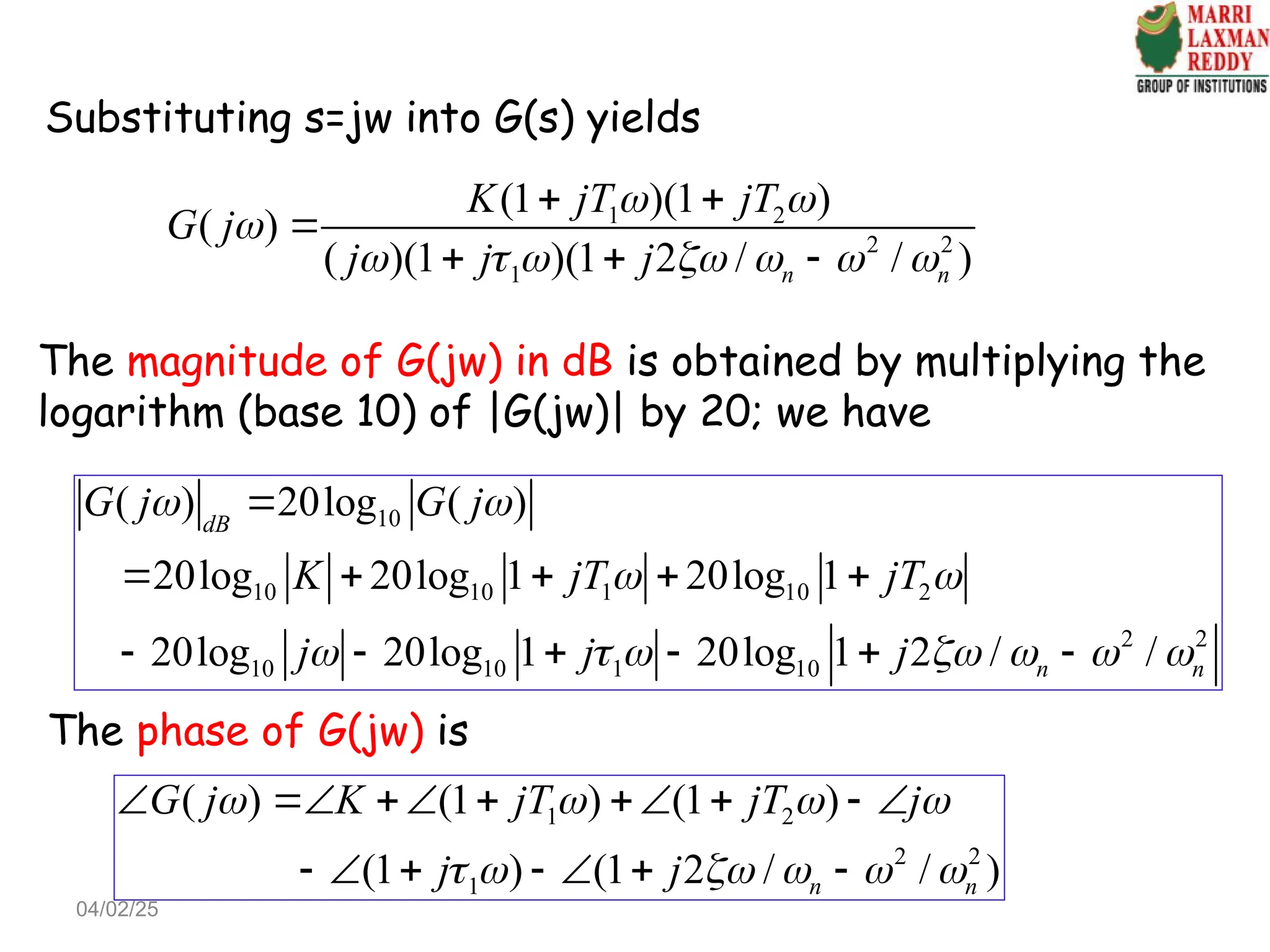
Chapter 4 discusses frequency-domain analysis, focusing on frequency response and its significance in feedback control system design. The chapter outlines the advantages of using frequency-response methods, including the ability to work with uncertain plant models and utilize experimental data for design without complex data processing. It also covers key concepts such as transfer functions, gain-phase characteristics, and the Nyquist criterion for determining stability in closed-loop systems.


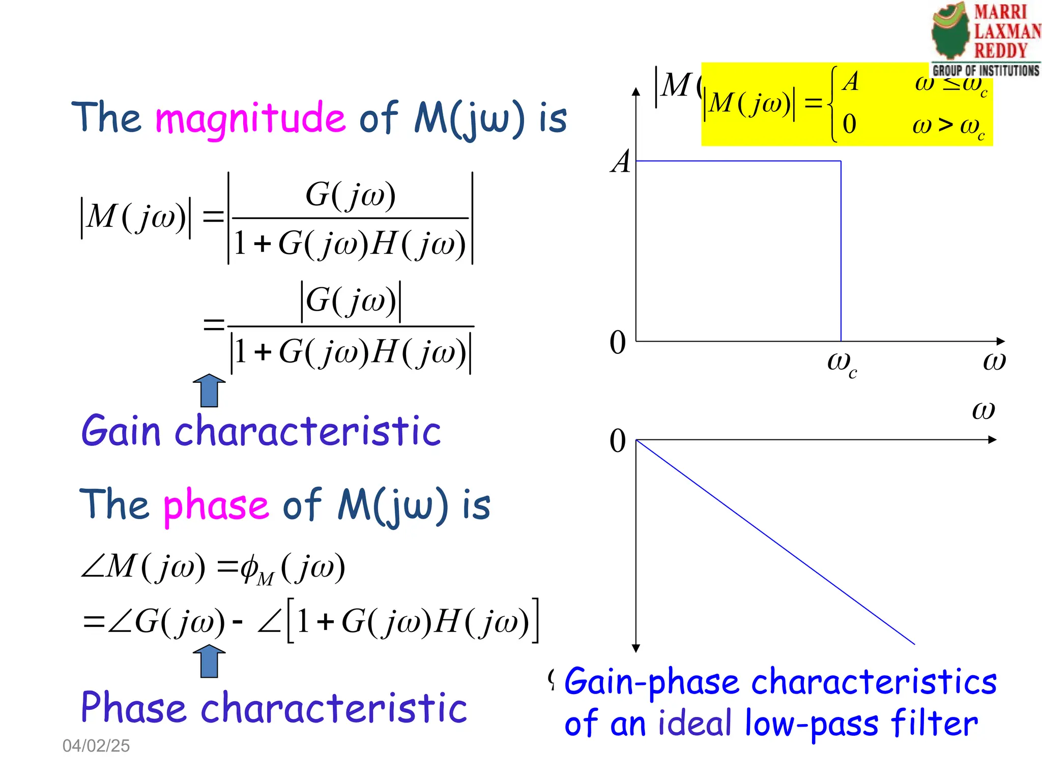
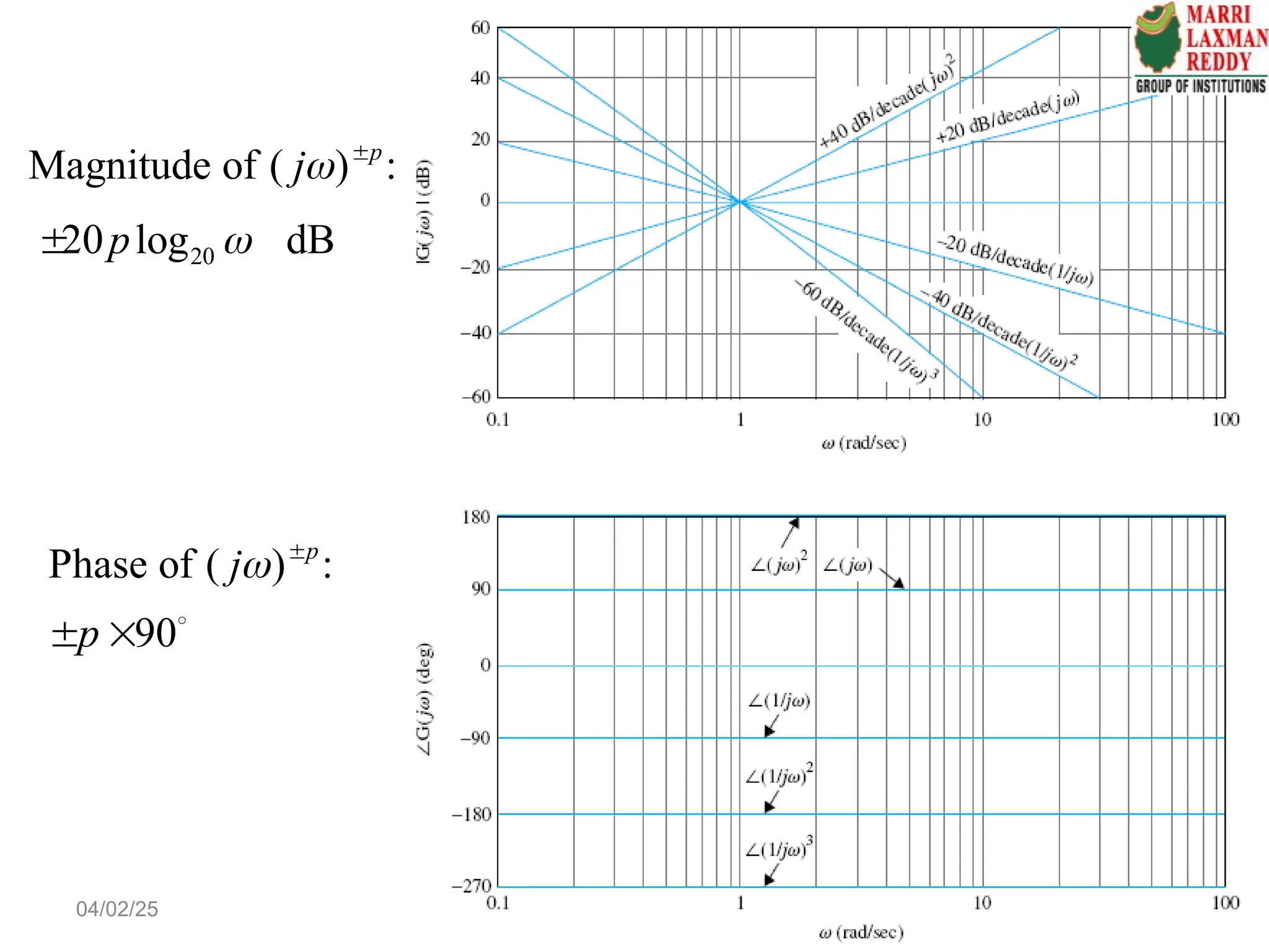
![The magnitude of M(ju) is
2 2 2 1/2
1
( )
[(1 ) (2 ) ]
M ju
u u
The phase of M(ju) is
1
2
2
( ) ( ) tan
1
M
u
M j j
u
The resonant frequency of M(ju) is
( )
0
d M ju
du
2
1 2
r
u
With , we have
r r n
u
2
1 2
r n
Since frequency is a real quantity, it requires 2
1 2 0
So 0.707
2
1
2 1
r
M
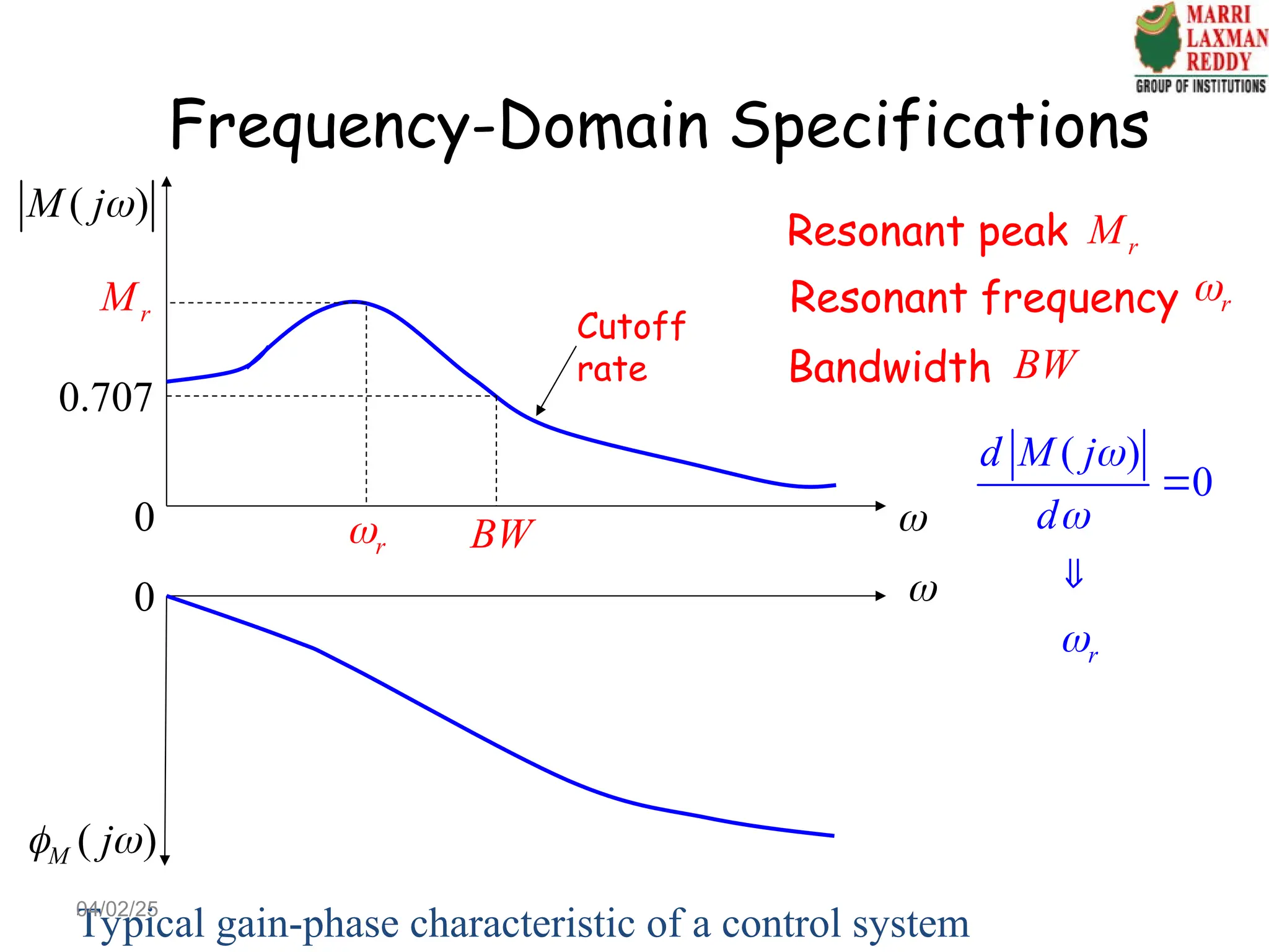
Resonant peak
04/02/25](https://image.slidesharecdn.com/555328898-unit-4-1-ppt-cs-250204034236-5724e0e0/75/555328898-Unit-4-1-PPT-CS-ppt-introduction-12-2048.jpg)
![According to the definition of Bandwidth
2 2 2 1/2
1 1
( ) 0.707
[(1 ) (2 ) ] 2
M ju
u u
2 2 4 2
(1 2 ) 4 4 2
u
With , we have
n
u
2 4 2 1/2
[(1 2 ) 4 4 2]
n
BW
04/02/25](https://image.slidesharecdn.com/555328898-unit-4-1-ppt-cs-250204034236-5724e0e0/75/555328898-Unit-4-1-PPT-CS-ppt-introduction-13-2048.jpg)
![Resonant peak
2
1
2 1
r
M
Resonant frequency
2
1 2
r n
For a prototype second-order system ( )
0.707
Bandwidth
2 4 2 1/2
[(1 2 ) 4 4 2]
n
BW
depends on only.
For 0, the system is unstable;
For 0< 0.707, ;
For 0.707, 1
r
r
r
M
M
M
depends on both and .
For 0< 0.707, fixed, ;
For 0.707, 0.
r n
n r
r
is directly proportional to ,
For 0 0.707, fixed, ;
n n
n
n
BW BW
BW
BW
04/02/25](https://image.slidesharecdn.com/555328898-unit-4-1-ppt-cs-250204034236-5724e0e0/75/555328898-Unit-4-1-PPT-CS-ppt-introduction-14-2048.jpg)
![Correlation between pole locations, unit-step response and
the magnitude of the frequency response
2
2 2
2
n
n n
s s
( )
r t ( )
y t
0 1
j
0
n
1
cos
0
( )
M j
0dB
0.3dB
BW
2 4 2 1/2
[(1 2 ) 4 4 2]
n
BW
2
1 0.4167 2.917
r
n
t
0
( )
y t
1.0
0.9
0.1 t
2
/ 1
max overshoot e
04/02/25](https://image.slidesharecdn.com/555328898-unit-4-1-ppt-cs-250204034236-5724e0e0/75/555328898-Unit-4-1-PPT-CS-ppt-introduction-15-2048.jpg)
![Resonant peak
2
(
1
2 1
0.707)
r
M
0.6
18
n
For 0< 0.707, ;
For 0.707, 1
r
r
M
M
1 1.04
r
M
0.6
Bandwidth
2 4 2 1/2
[(1 2 ) 4 4 2]
n
BW
is directly proportional to ,
For 0 0.707, fixed, ;
n n
n
n
BW BW
BW
BW
0.6 0.707
1 1.15
n
BW
1.15
n n
BW
18
n
18
BW
Based on time-domain analysis, we obtain and
Frequency-domain specifications:
04/02/25](https://image.slidesharecdn.com/555328898-unit-4-1-ppt-cs-250204034236-5724e0e0/75/555328898-Unit-4-1-PPT-CS-ppt-introduction-17-2048.jpg)

![Mapping from the complex s-plane to the
Δ(s) -plane
Exercise 1: Consider a function Δ(s) =s-1, please map a
circle with a radius 1 centered at 1 from s-plane to the
Δ(s)-plane .
1 2
3 4
2; 1
0; 1
s s j
s s j
1 2
3 4
( ) 1; ( )
( ) 1; ( )
s s j
s s j
Δ( s)-plane
Im
j
Re[ ( )]
s
1
( )
s
2
( )
s
3
( )
s
4
( )
s
0
1
s-plane
j
1
s
2
s
3
s
4
s
2
1
1
0
Mapping
04/02/25](https://image.slidesharecdn.com/555328898-unit-4-1-ppt-cs-250204034236-5724e0e0/75/555328898-Unit-4-1-PPT-CS-ppt-introduction-28-2048.jpg)
![-2 -1 0 1 2 3 4 5
-4
-3
-2
-1
0
1
2
3
4
Nyquist Diagram
Real Axis
Imaginary
Axis
An example
Consider the system with
the loop function
3
5
( ) ( )
( 1)
G s H s
s
Matlab program for
Nyquist plot
(G(s)H(s) plot)
>>num=5;
>>den=[1 3 3 1];
>>nyquist(num,den);
Question 1: is the
closed-loop system
stable?
Question 2: what if
3
5
( ) ( ) ?
( 1)
K
G s H s
s
N=0, P=0,
N=-P, stable
04/02/25](https://image.slidesharecdn.com/555328898-unit-4-1-ppt-cs-250204034236-5724e0e0/75/555328898-Unit-4-1-PPT-CS-ppt-introduction-35-2048.jpg)
![Root Locus
Real Axis
Imaginary
Axis
-4 -3 -2 -1 0 1 2
-3
-2
-1
0
1
2
3
*
3 3
5 1
( ) ( )
( 1) ( 1)
K
G s H s K
s s
1. With root locus technique:
For K* varies from 0
to ∞, we draw the RL
>>num=1;
>>den=[1 3 3 1];
>>rlocus(num,den);
When K*=8
(K=1.6), the RL
cross the jw-axis,
the closed-loop
system is
marginally stable.
For K*>8 (K>1.6), the closed-loop system has two roots in
the RHP and is unstable.
*
K
*
K
*
K
*
0
K
*
8
K
04/02/25](https://image.slidesharecdn.com/555328898-unit-4-1-ppt-cs-250204034236-5724e0e0/75/555328898-Unit-4-1-PPT-CS-ppt-introduction-36-2048.jpg)
![2. With Nyquist plot and
Nyquist criterion:
-2 -1 0 1 2 3 4 5
-4
-3
-2
-1
0
1
2
3
4
Nyquist Diagram
Real Axis
Imaginary
Axis
>>K=1;
>>num=5*K;
>>den=[1 3 3 1];
>>nyquist(num,den);
Nyquist plot
does not
encircle (-1,j0),
so N=0
K=1
3
5
( ) ( )
( 1)
K
G s H s
s
No pole of
G(s)H(s) in
RHP, so P=0;
Thus N=-P
The closed-loop system is stable
04/02/25](https://image.slidesharecdn.com/555328898-unit-4-1-ppt-cs-250204034236-5724e0e0/75/555328898-Unit-4-1-PPT-CS-ppt-introduction-37-2048.jpg)
![-2 -1 0 1 2 3 4 5 6 7 8
-6
-4
-2
0
2
4
6
Nyquist Diagram
Real Axis
Imaginary
Axis
2. With Nyquist plot and
Nyquist criterion:
>>K=1.6;
>>num=5*K;
>>den=[1 3 3 1];
>>nyquist(num,den);
The Nyquist plot
just go through
(-1,j0)
K=1.6
3
5
( ) ( )
( 1)
K
G s H s
s
No pole of
G(s)H(s) in RHP,
so P=0;
The closed-loop system is marginally stable
04/02/25](https://image.slidesharecdn.com/555328898-unit-4-1-ppt-cs-250204034236-5724e0e0/75/555328898-Unit-4-1-PPT-CS-ppt-introduction-38-2048.jpg)
![-5 0 5 10 15 20
-15
-10
-5
0
5
10
15
Nyquist Diagram
Real Axis
Imaginary
Axis
2. With Nyquist plot and
Nyquist criterion:
>>K=4;
>>num=5*K;
>>den=[1 3 3 1];
>>nyquist(num,den);
Nyquist plot
encircles (-1,j0)
twice, so N=2
K=4
3
5
( ) ( )
( 1)
K
G s H s
s
No pole of
G(s)H(s) in RHP,
so P=0;
Thus Z=N+P=2
The closed-loop system has two poles in RHP and is unstable
04/02/25](https://image.slidesharecdn.com/555328898-unit-4-1-ppt-cs-250204034236-5724e0e0/75/555328898-Unit-4-1-PPT-CS-ppt-introduction-39-2048.jpg)
![Example Consider a single-loop feedback system with the
loop transfer function
( ) ( ) ( )
( 2)( 10)
K
L s G s H s
s s s
Analyze the stability of the closed-loop system.
Solution.
Since L(s) is minimum-phase, we can analyze the closed-loop
stability by investigating whether the Nyquist plot enclose
the critical point (-1,j0) for L(jw)/K first.
( ) 1
( 2)( 10)
L j
K j j j
w=∞:
( )
0 270
L j
K
w=0+
:
( 0)
90
L j
K
0
Im
j
Real
0
Im[ ( ) ] 0
L j K
04/02/25](https://image.slidesharecdn.com/555328898-unit-4-1-ppt-cs-250204034236-5724e0e0/75/555328898-Unit-4-1-PPT-CS-ppt-introduction-44-2048.jpg)
![1
Im[ ( ) ] Im[ ] 0
( 2)( 10)
L j K
j j j
20 /
rad s
The frequency is positive, so 20 /
rad s
1
( 20) 0.004167
20( 20 2)( 20 10)
L j K
j j j
1. 240 ( 20) 1
K L j
the Nyquist plot does not enclose (-1,jw);
2. 240 ( 20) 1
K L j
the Nyquist plot goes through (-1,jw);
3. 240 ( 20) 1
K L j
the Nyquist plot encloses (-1,jw).
stable
marginally stable
unstable
04/02/25](https://image.slidesharecdn.com/555328898-unit-4-1-ppt-cs-250204034236-5724e0e0/75/555328898-Unit-4-1-PPT-CS-ppt-introduction-45-2048.jpg)
![-30 -25 -20 -15 -10 -5 0 5 10
-20
-15
-10
-5
0
5
10
15
20
Root Locus
Real Axis
Imaginary
Axis
1
( ) ( ) ( )
( 2)( 10)
L s G s H s K
s s s
>>z=[]
>>p=[0, -2, -10];
>>k=1
>>sys=zpk(z,p,k);
>>rlocus(sys);
240
K
By root locus technique
04/02/25](https://image.slidesharecdn.com/555328898-unit-4-1-ppt-cs-250204034236-5724e0e0/75/555328898-Unit-4-1-PPT-CS-ppt-introduction-46-2048.jpg)
![If the Nyquist plot of G(jw) intersects with the real axis, we have
Im[ ( )] 0
G j
2
4 2 4 2
10 10 10
( )
( 1)
G j j
j j
4 2
10
0
This means that the G(jw) plot intersects only with the real axis of the
G(jw)-plane at the origin.
Similarly, intersection of G(jw) with the imaginary axis:
which corresponds to the origin of the G(jw)-plane.
The conclusion is that the Nyquist
plot of G(jw) does not intersect any
one of the axes at any finite
nonzero frequency.
Re[ ( )] 0
G j
At w=0, Re[ ( )] 10
G j
At w=∞, Re[ ( )] 0
G j
04/02/25](https://image.slidesharecdn.com/555328898-unit-4-1-ppt-cs-250204034236-5724e0e0/75/555328898-Unit-4-1-PPT-CS-ppt-introduction-52-2048.jpg)
![Example Consider a system with a loop transfer function as
2500
( )
( 5)( 50)
L s
s s s
Determine its gain margin and phase margin.
Solution. Phase crossover frequency ωp:
Im[ ( )] 0 15.88 rad/sec
p
L j
10
GM = 20log ( ) 14.80 dB
p
L j
Gain margin:
Gain crossover frequency ωg:
( ) 1 6.22 rad/sec
g g
L j
Phase margin:
PM = ( ) 180 31.72
g
L j
0
Im
j
0
1
( ) 0.182
p
L j 15.88
p
6.22
g
31.72
0.182
04/02/25](https://image.slidesharecdn.com/555328898-unit-4-1-ppt-cs-250204034236-5724e0e0/75/555328898-Unit-4-1-PPT-CS-ppt-introduction-53-2048.jpg)

![4. Complex poles and zeros
Consider the second-order transfer function
2
2 2 2 2
1
( )
2 1 (2 ) (1 )
n
n n n n
G s
s s s s
We are interested only in the case when ζ ≤ 1, since
otherwise G(s) would have two unequal real poles, and
the Bode plot can be obtained by considering G(s) as the
product of two transfer functions with simple poles.
By letting s=jw, G(s) becomes
2 2
1
( )
[1 ( )] 2 ( )
n n
G j
j
04/02/25](https://image.slidesharecdn.com/555328898-unit-4-1-ppt-cs-250204034236-5724e0e0/75/555328898-Unit-4-1-PPT-CS-ppt-introduction-67-2048.jpg)
![2 2
1
( )
[1 ( )] 2 ( )
n n
G j
j
The magnitude of G(jw) in dB is
10
2 2 2 2 2
10
( ) 20log ( )
20log [1 ( )] 4 ( )
dB
n n
G j G j
At very low frequencies, / 1
n
10
( ) 20log 1 0 dB
dB
G j
At very high frequencies, / 1
n
4
10 10
( ) 20log ( ) 40log ( ) dB
n n
dB
G j
This equation represents a straight line with a slope of
40 dB decade in the Bode plot coordinates.
The two lines
intersect at:
n
(corner
frequency)
04/02/25](https://image.slidesharecdn.com/555328898-unit-4-1-ppt-cs-250204034236-5724e0e0/75/555328898-Unit-4-1-PPT-CS-ppt-introduction-68-2048.jpg)


![Circuit Network Analysis - [Chapter5] Transfer function, frequency response, ...](https://cdn.slidesharecdn.com/ss_thumbnails/ch5-150613063859-lva1-app6891-thumbnail.jpg?width=640&height=640&fit=bounds)