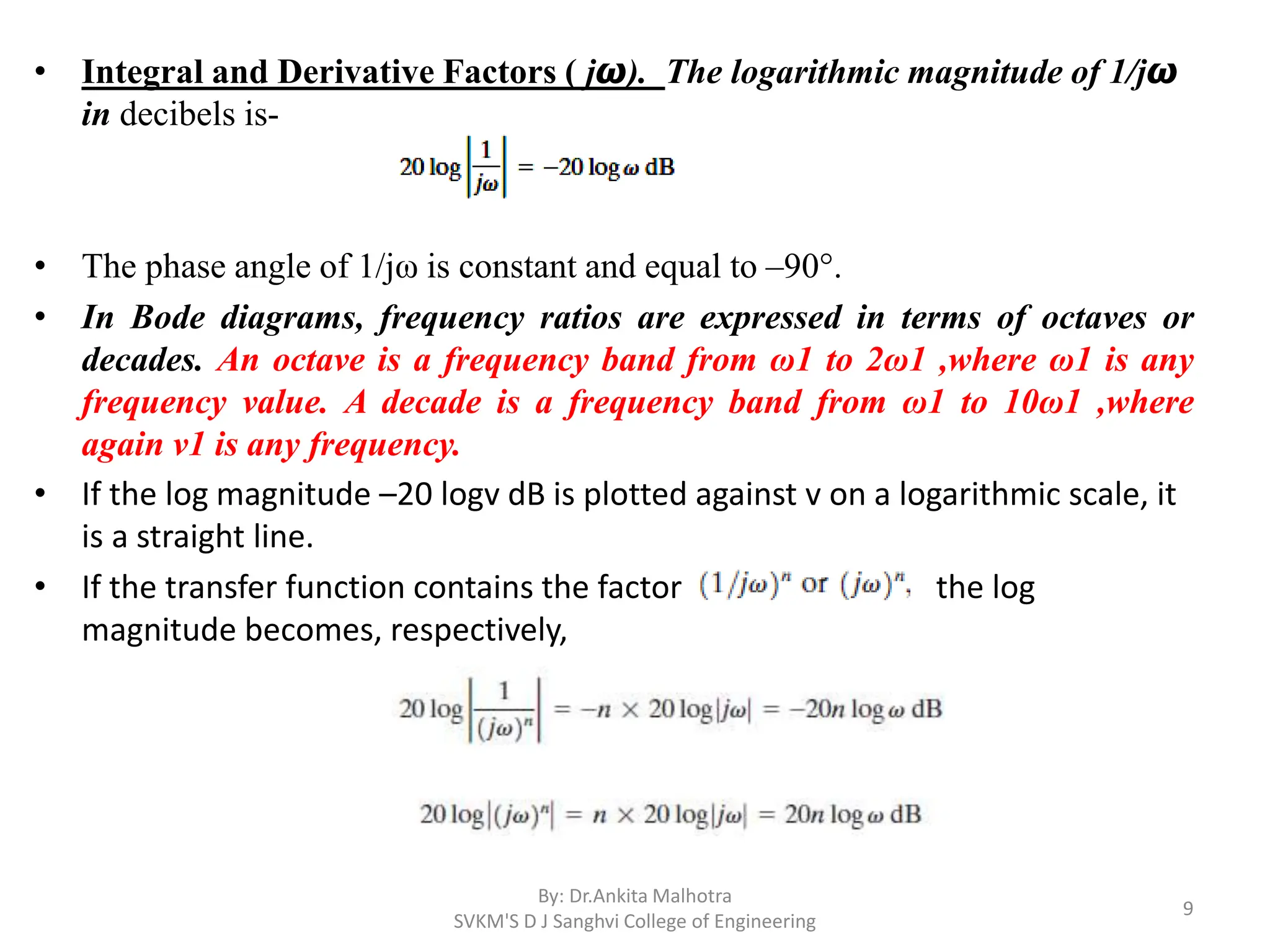
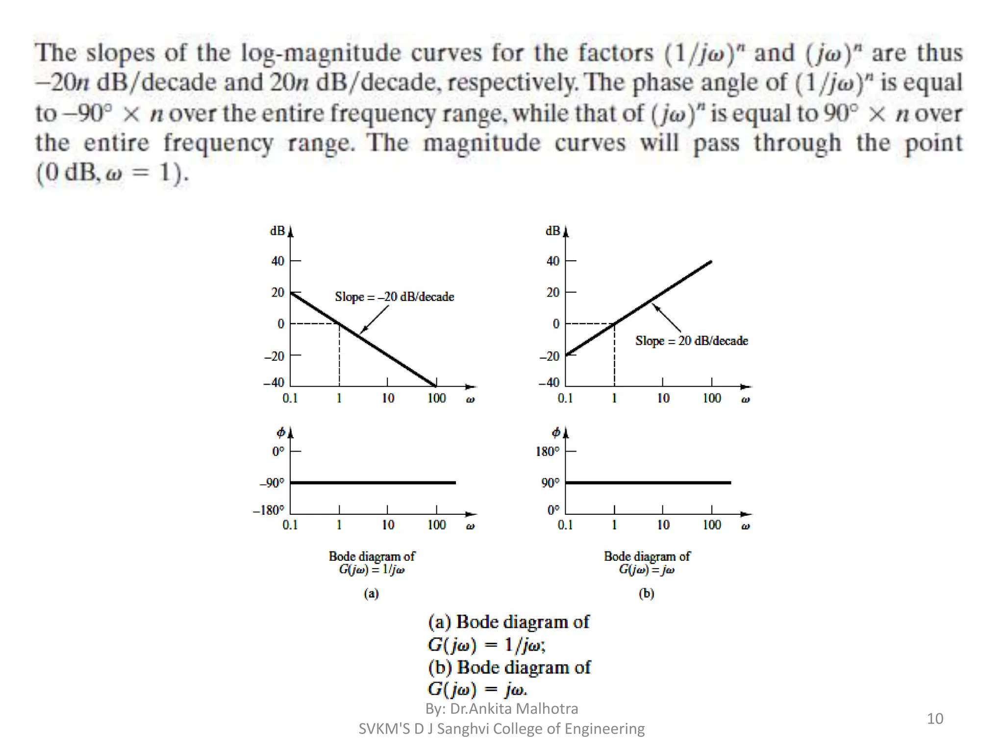
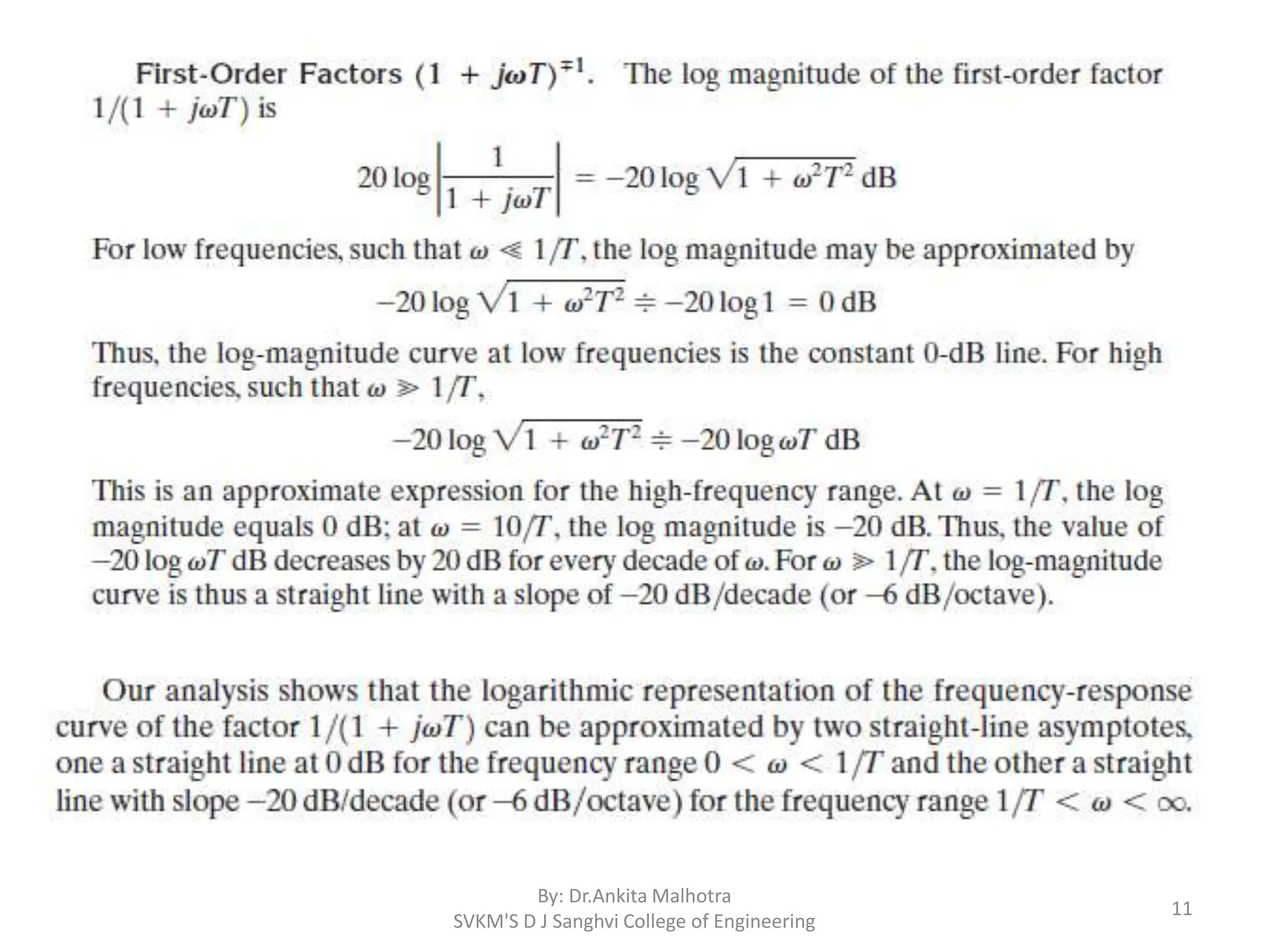
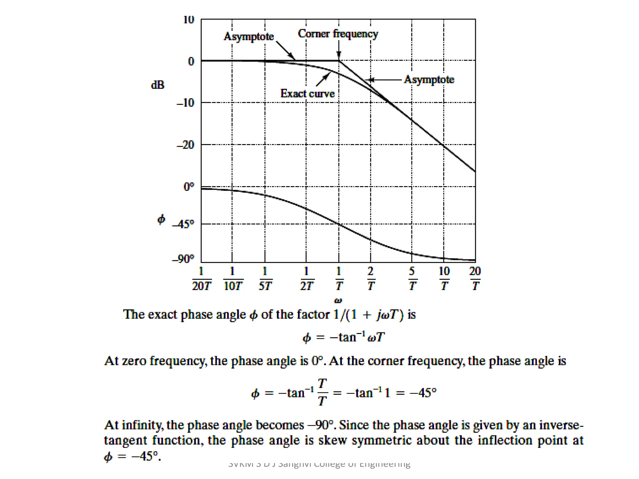
The document provides an overview of stability analysis in control systems using frequency response methods, explaining the steady-state response of systems to sinusoidal inputs. It details the advantages of frequency-response tests, how to obtain steady-state outputs, and introduces Bode diagrams for logarithmic plotting of transfer functions. Additionally, it discusses the Nyquist stability criterion for evaluating the stability of closed-loop systems based on open-loop frequency responses.
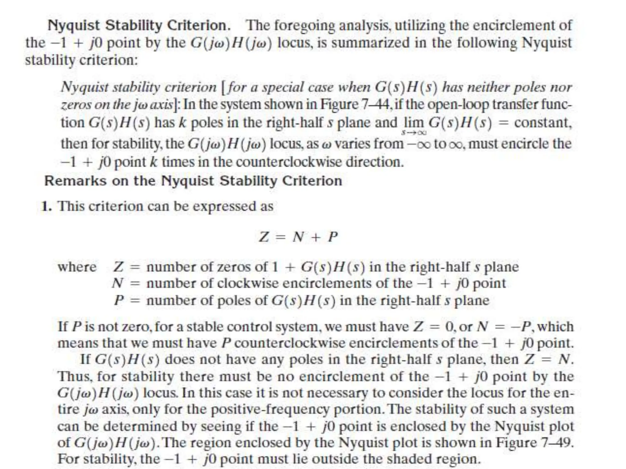
![Nyquist criteria
• The Nyquist stability criterion determines the stability of a closed-loop
system from its open-loop frequency response and open-loop poles.
• Let closed loop TF is
By: Dr.Ankita Malhotra
SVKM'S D J Sanghvi College of Engineering
23
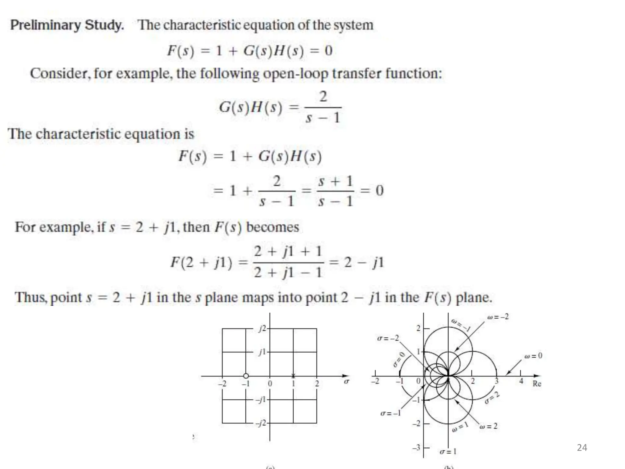
must lie in the left-half s plane. [It is noted that, although poles and zeros of the open-loop
transfer function G(s)H(s) may be in the right-half s plane, the system is stable if all the
poles of the closed-loop transfer function (that is, the roots of the characteristic equation)
are in the left-half s plane.] The Nyquist stability criterion relates the open-loop frequency
response G(jw)H(jw) to the number of zeros and poles of 1+G(s)H(s) that lie in the
right-half s plane.](https://image.slidesharecdn.com/unit6-240711151405-512c35dc/75/Stability-of-control-systems-in-frequency-domain-23-2048.jpg)


![Circuit Network Analysis - [Chapter5] Transfer function, frequency response, ...](https://cdn.slidesharecdn.com/ss_thumbnails/ch5-150613063859-lva1-app6891-thumbnail.jpg?width=640&height=640&fit=bounds)


