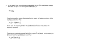
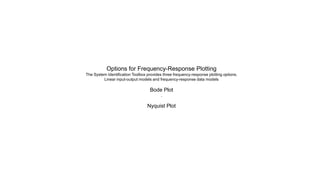
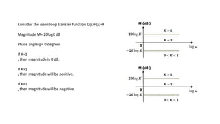
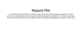
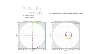
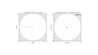
What Is Frequency
Response?
Frequency response plots show the complex values of a transfer function as a
function of frequency.
• In the case of linear dynamic systems, the transfer function G is essentially an operator
that takes the input u of a linear system to the output y:
Y =Gu
For a continuous-time system, the transfer function relates the Laplace transforms of the
input U(s) and output Y(s):
Y(s) = G(s)U(s)
In this case, the frequency function G(iω) is the transfer function evaluated on the
imaginary axis s=iω.
For a discrete-time system sampled with a time interval T, the transfer function relates the
Z-transforms of the input U(z) and output Y(z) :
Y(z)=G(z)U(z)
Frequency response plots provide insight into linear
systems dynamics, such as frequency-dependent gains,
resonances, and phase shifts. Frequency response plots
also contain information about controller requirements and
achievable bandwidths
Options for Frequency-Response Plotting
The System Identification Toolbox provides three frequency-response plotting options.
Linear input-output models and frequency-response data models
Bode Plot
.
Nyquist Plot
Bode Plot
A Bode plot is a graph commonly used in control system engineering to determine the stability of a
control system. A Bode plot maps the frequency response of the system through two graphs – the
Bode magnitude plot (expressing the magnitude in decibels) and the Bode phase plot (expressing the
phase shift in degrees).
In both the plots, x-axis represents angular frequency (logarithmic scale). Whereas y axis represents
the magnitude (linear scale) of open loop transfer function in the magnitude plot and the phase angle
(linear scale) of the open loop transfer function in the phase plot.
M=20log|G(jω)H(jω)|
The magnitude of the open loop transfer function in dB is
The phase angle of the open loop transfer function in
degrees is
ϕ=∠G(jω)H(jω)
Basic of Bode Plots
The following table shows the slope, magnitude and the phase angle values of the
terms present in the open loop transfer function. This data is useful while drawing the
Bode plots.
Consider the open loop transfer function G(s)H(s)=K
Magnitude M= 20logK dB
Phase angle ϕ= 0 degrees
If K=1
, then magnitude is 0 dB.
If K>1
, then magnitude will be positive.
If K<1
, then magnitude will be negative.
The measured phase at 0 dB is -135°, so the phase
margin is 45°. The gain at -180° degrees is -9 dB, so the
gain margin is 9 dB. Since phase margin is positive, this
system is stable.
The measured gain is +13 dB when phase is -180°, so the
gain margin is -13 dB. At a gain of 0 dB, the measured
phase is minus 215°, so the phase margin is minus 35° at
the gain crossover point. This system is unstable.
Stable and unstable closed loop
systems
Nyquist Plot
is a parametric plot of a frequency response used in automatic control and signal processing. The most
common use of Nyquist plots is for assessing the stability of a system with feedback. In Cartesian coordinates,
the real part of the transfer function is plotted on the X-axis while the imaginary part is plotted on the Y-axis.
This has roots at s= -4.5 ± 9.4j so the system is stable
There are no poles of L(s) in the right half plane. This
means that the characteristic equation of the closed loop
transfer function has no zeros in the right half plane (the
closed loop transfer function has no poles there). The
system is stable.
frequency response

frequency response

  • 1.
    What Is Frequency Response? Frequencyresponse plots show the complex values of a transfer function as a function of frequency.
  • 2.
    • In thecase of linear dynamic systems, the transfer function G is essentially an operator that takes the input u of a linear system to the output y: Y =Gu For a continuous-time system, the transfer function relates the Laplace transforms of the input U(s) and output Y(s): Y(s) = G(s)U(s) In this case, the frequency function G(iω) is the transfer function evaluated on the imaginary axis s=iω. For a discrete-time system sampled with a time interval T, the transfer function relates the Z-transforms of the input U(z) and output Y(z) : Y(z)=G(z)U(z)
  • 3.
    Frequency response plotsprovide insight into linear systems dynamics, such as frequency-dependent gains, resonances, and phase shifts. Frequency response plots also contain information about controller requirements and achievable bandwidths
  • 4.
    Options for Frequency-ResponsePlotting The System Identification Toolbox provides three frequency-response plotting options. Linear input-output models and frequency-response data models Bode Plot . Nyquist Plot
  • 5.
    Bode Plot A Bodeplot is a graph commonly used in control system engineering to determine the stability of a control system. A Bode plot maps the frequency response of the system through two graphs – the Bode magnitude plot (expressing the magnitude in decibels) and the Bode phase plot (expressing the phase shift in degrees). In both the plots, x-axis represents angular frequency (logarithmic scale). Whereas y axis represents the magnitude (linear scale) of open loop transfer function in the magnitude plot and the phase angle (linear scale) of the open loop transfer function in the phase plot. M=20log|G(jω)H(jω)| The magnitude of the open loop transfer function in dB is The phase angle of the open loop transfer function in degrees is ϕ=∠G(jω)H(jω)
  • 6.
    Basic of BodePlots The following table shows the slope, magnitude and the phase angle values of the terms present in the open loop transfer function. This data is useful while drawing the Bode plots.
  • 7.
    Consider the openloop transfer function G(s)H(s)=K Magnitude M= 20logK dB Phase angle ϕ= 0 degrees If K=1 , then magnitude is 0 dB. If K>1 , then magnitude will be positive. If K<1 , then magnitude will be negative.
  • 8.
    The measured phaseat 0 dB is -135°, so the phase margin is 45°. The gain at -180° degrees is -9 dB, so the gain margin is 9 dB. Since phase margin is positive, this system is stable. The measured gain is +13 dB when phase is -180°, so the gain margin is -13 dB. At a gain of 0 dB, the measured phase is minus 215°, so the phase margin is minus 35° at the gain crossover point. This system is unstable. Stable and unstable closed loop systems
  • 9.
    Nyquist Plot is aparametric plot of a frequency response used in automatic control and signal processing. The most common use of Nyquist plots is for assessing the stability of a system with feedback. In Cartesian coordinates, the real part of the transfer function is plotted on the X-axis while the imaginary part is plotted on the Y-axis.
  • 10.
    This has rootsat s= -4.5 ± 9.4j so the system is stable
  • 11.
    There are nopoles of L(s) in the right half plane. This means that the characteristic equation of the closed loop transfer function has no zeros in the right half plane (the closed loop transfer function has no poles there). The system is stable.