The document discusses frequency response analysis, emphasizing the steady state response of systems to sinusoidal signals and the advantages of frequency analysis for stability estimation and practical testing. Key concepts include resonant peak, resonant frequency, bandwidth, gain margin, and phase margin, along with various frequency response plots such as Bode, Nyquist, and Nichols. The document also provides formulas and examples for calculating gain and drawing Bode plots for different transfer functions.

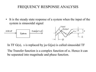
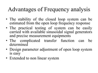
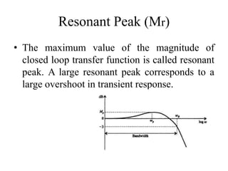
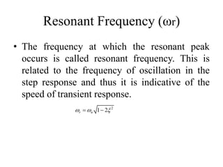
1. Frequency Response Analysis
Unit III

2. FREQUENCY RESPONSE ANALYSIS
• It is the steady state response of a system when the input of the
system is sinusoidal signal
In TF G(s), s is replaced by jω G(jω) is called sinusoidal TF
The Transfer function is a complex function of ω. Hence it can
be separated into magnitude and phase function.

3. Advantages of Frequency analysis
• The stability of the closed loop system can be
estimated from the open loop frequency response
• The practical testing of system can be easily
carried with available sinusoidal signal generators
and precise measurement equipments
• The complicated transfer function can be
determined
• Design parameter adjustment of open loop system
is easy
• Extended to non linear system

4. Frequency domain specifications
• Resonant Peak (Mr)
• Resonant Frequency (ωr)
• Bandwidth (ωb)
• Cut-off rate
• Gain margin (Kg)
• Phase margin(γ)

5. Frequency Response Plots
• Bode Plot
• Polar Plot
• Nyquist plot
• Nichols Plot
• M and N circles
• Nichols Chart

6. Resonant Peak (Mr)
• The maximum value of the magnitude of
closed loop transfer function is called resonant
peak. A large resonant peak corresponds to a
large overshoot in transient response.

7. Resonant Frequency (ωr)
• The frequency at which the resonant peak
occurs is called resonant frequency. This is
related to the frequency of oscillation in the
step response and thus it is indicative of the
speed of transient response.
2
1 2
r n
  
 

8. Bandwidth (ωb)
• The bandwidth is the range of frequencies for
which the system normalized gain is more than
-3dB
• The frequency at which the gain is -3dB is
called cut-off frequency.

9. Cut-off Rate
• The slope of the log magnitude curve near the
cut off frequency is called cut-off rate.
• The cut-off rate indicates the stability of
system to distinguish the signal from noise

10. Gain Margin (Kg)
• The gain margin is the factor by which the
system gain can be increased to drive it to the
verge of instability.
• It may be defined as the reciprocal of the gain
at the phase cross over frequency (pc). The
phase cross over frequency is the frequency at
which the phase is 180.
1
( )
pc
Kg
G j


11. Phase Margin (γ)
• The phase margin is defined as the amount of
additional phase lag at the gain crossover
frequency (gc) required to bring the system to
the verge of instability.
Phase margin  = gc + 180 Where gc =  G (j) H (j) at  = gc

13. Polar Graph

16. Corner frequencies wc1 = 0.5 rad/sec and wc2 = 1 rad/sec

21. The corner frequency is

23. Bode Plot
• Frequency response plot
• Magnitude Vs logw
• Phase angle Vs logw

24. Bode Plot
Calculate the gain in dB for lowest frequency and first corner frequency
Calculate the gain using the below formulae for all other frequency

25. Draw the bode plot for the transfer function and find
gain cross over and phase cross over frequencies
)]
1
1
.
0
)(
4
.
0
1
(
[
10
)
(



s
s
s
s
G

30. Sketch the Bode plot for the following transfer function and
obtain gain margin and phase margin
)]
5
3
(
[
1
)
( 2



s
s
s
s
G

33. Sketch the bode plot and hence find gain cross over frequency,
phase cross over frequency, gain margin and phase margin for
the function
.
)
100
4
)(
2
(
)
3
(
10
)
( 2





s
s
s
s
s
s
G