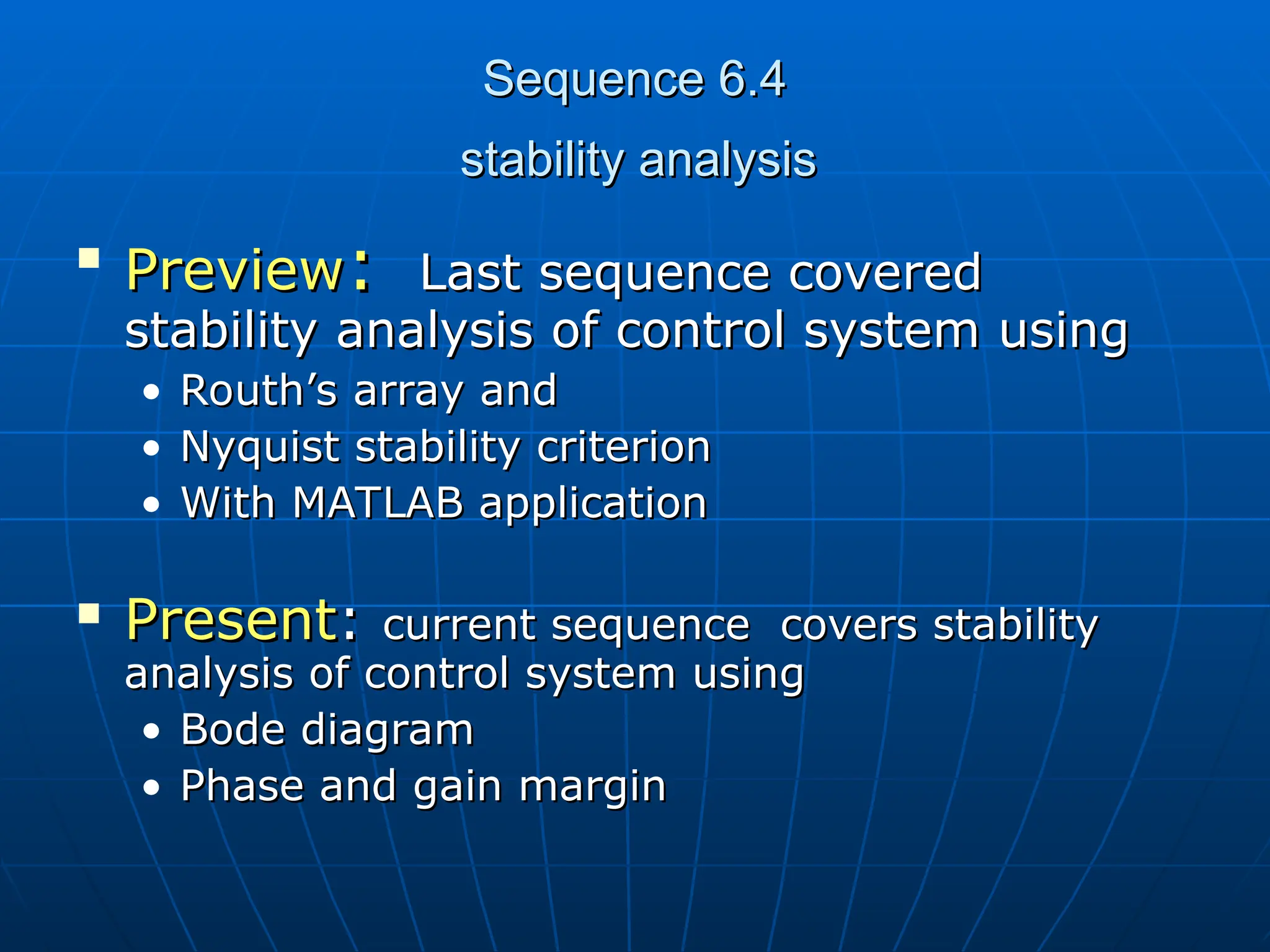
The document discusses stability analysis of control systems using Bode plots, including phase and gain margins, as well as relevant MATLAB applications. It explains how to create Bode diagrams, determine bandwidth, and analyze various system elements such as integrators and derivatives. The document also provides MATLAB code for plotting and assessing system stability.

1. Session-6
Session-6
automatic control
automatic control
systems
systems
Dr. Saber Abdrabbo
Dr. Saber Abdrabbo

2. Sequence 6.4
Sequence 6.4
stability analysis
stability analysis

Preview
Preview:
: Last
Last sequence covered
sequence covered
stability analysis of control system using
stability analysis of control system using
• Routh’s array and
Routh’s array and
• Nyquist stability criterion
Nyquist stability criterion
• With MATLAB application
With MATLAB application
 Present
Present:
: current sequence covers stability
current sequence covers stability
analysis of control system using
analysis of control system using
• Bode diagram
Bode diagram
• Phase and gain margin
Phase and gain margin

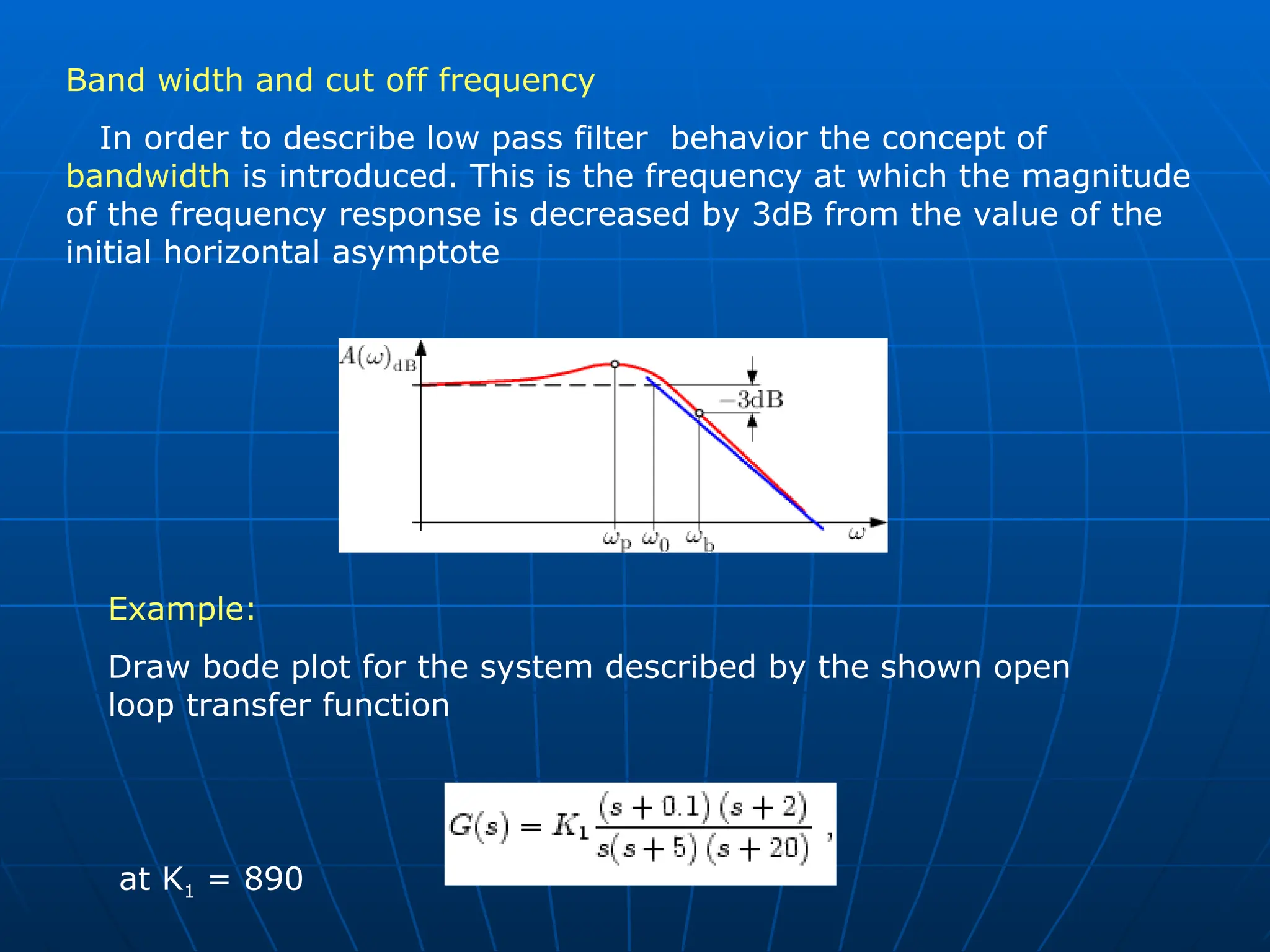
3. If the absolute value and the phase of the frequency response are separately
plotted over the frequency on semi log paper . This representation is called a
Bode diagram or Bode plot. Usually will be specified in decibels [dB] By
definition this is
Bode plot
Decade
General form of transfer
)
(
)
(
)
(
1
1
j
n
j
v
i
m
i
p
s
s
z
s
K
s
G







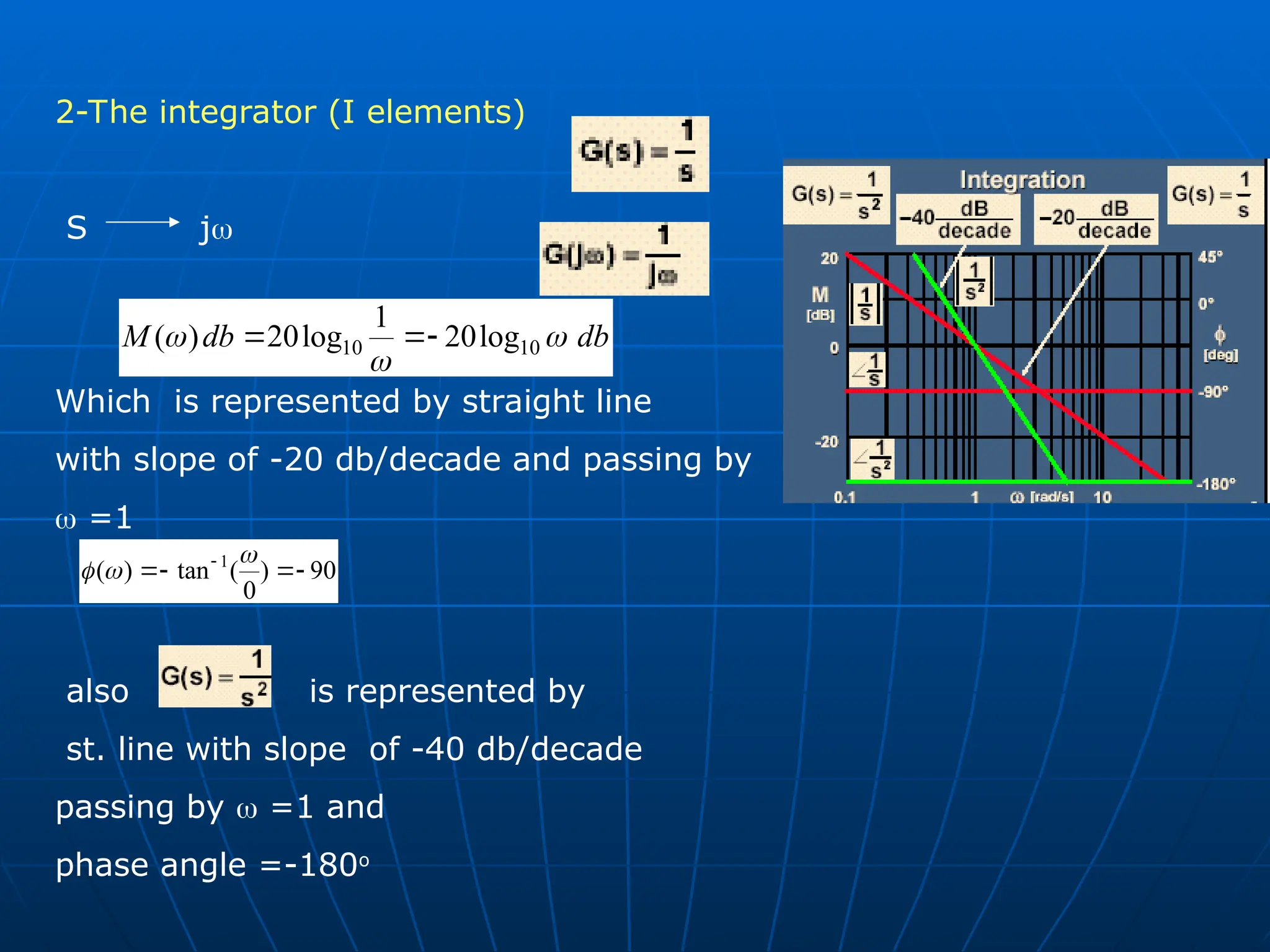
1-Gain element (K)
S j
0
)
0
(
tan
)
( 1

 
K


and
t
cons
db
K
K
db
M tan
log
20
)
( 10 



M

4. 2-The integrator (I elements)
S j
Which is represented by straight line
with slope of -20 db/decade and passing by
 =1
also is represented by
st. line with slope of -40 db/decade
passing by  =1 and
phase angle =-180o
db
db
M 

 10
10 log
20
1
log
20
)
( 


90
)
0
(
tan
)
( 1



  



5. 3-Derivative elements (D elements)
Which is represented by straight line
with slope of 20 db/decade and passing by
 =1
also
G(S)=S2
is represented by
st. line with slope of 40 db/decade
passing by  =1 and
phase angle =180o


 j
j
G
j
S
S
S
G



)
(
)
(
90
)
0
(
tan
)
( 1


  


db
db
M 

 10
10 log
20
log
20
)
( 


6. 4-Real integrator (First order lag element )
and
and
for
For
Which is represented by straight line
starts at corner( ) with
slope of -20 db/decade
Phase angle changes from 0 to -90o
difference between approximated and real curve


1

c




10
1
1
.
0

c
-3db

7. 5-First order lead element( Proportional (P) +D( derivative))
is represented by straight line
starts at corner( ) with
slope of 20 db/decade
Phase angle changes from 0 to 90o
)
1
(
)
( 
 S
S
G 


1

c
6-2nd
order lag element
is represented by straight line
starts at corner freq. ( )
with resonance peak of
and slope of -40 db/decade
Phase angle changes from 0 to -180o
2
2
1 

 
 n
r
2
1
2
1

 

r
M

8. Band width and cut off frequency
In order to describe low pass filter behavior the concept of
bandwidth is introduced. This is the frequency at which the magnitude
of the frequency response is decreased by 3dB from the value of the
initial horizontal asymptote
Example:
Draw bode plot for the system described by the shown open
loop transfer function
at K1 = 890

9. Solution
The system which has only real poles and zeros
Rearrange the system into the form
K2=5 db
This system can now be decomposed into
Element
Element Slope
Slope Net
Net
slope
slope
comments
comments
1/S
1/S -20
-20 -20
-20 Passing by
Passing by

c
c=1
=1
20
20 0
0 
c
c=0.1
=0.1
20
20 20
20 
c
c=2
=2
-20
-20 0
0 
c
c=5
=5
-20
-20 -20
-20 
c
c=20
=20
Draw bode plot at K=1 according
to the following steps
1-Draw vertical lines for corner
frequencies
2-sort in ascending the elements
according to corner frequencies
3-draw each element
4- draw super composed curve
1
1
.
0

S
1
5
1

S
1
2

S
1
20
1

S

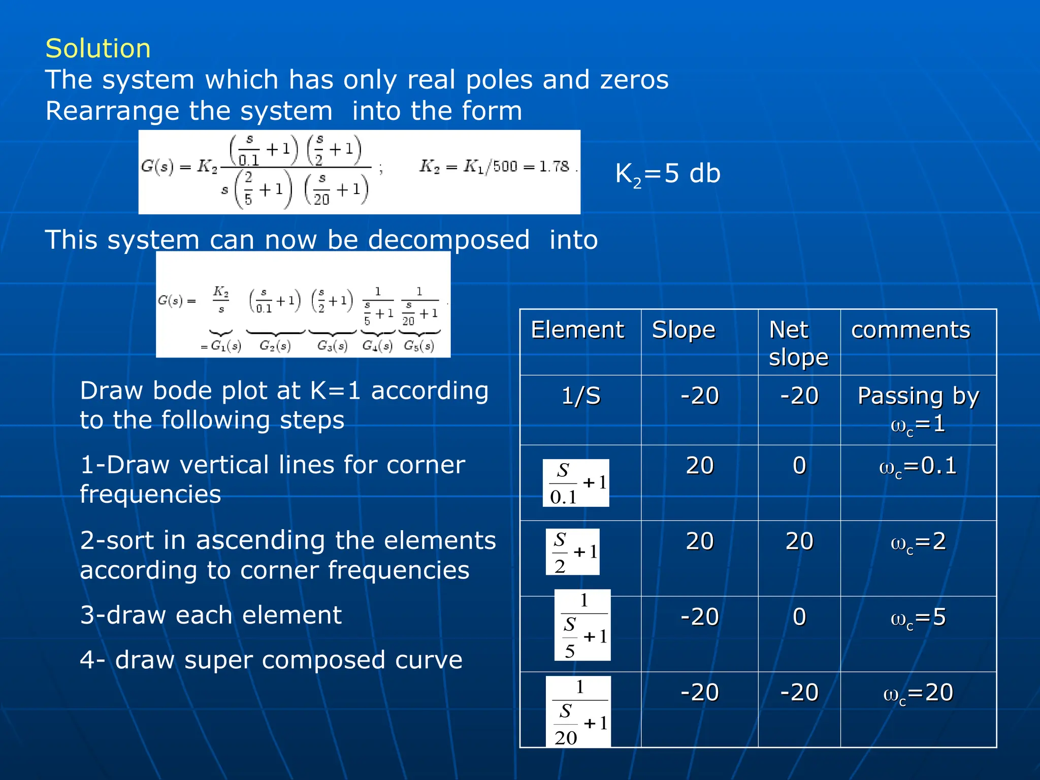
10. K=1
K=1.78
5 db
5-Shift bode plot at k=1 by 5 db
6-Draw the relation between phase
and frequencies according to the
following phase equation
20
tan
tan
2
tan
1
.
0
tan
90
)
( 1
5
1
1
1 



  









Following MATLAB code can be
written to draw the bode plot
for previous problem
Num=[8.9 18.69 1.78];
Den=[ 0.01 0.25 1 0];
sys=tf(num,den);
Bode(sys)

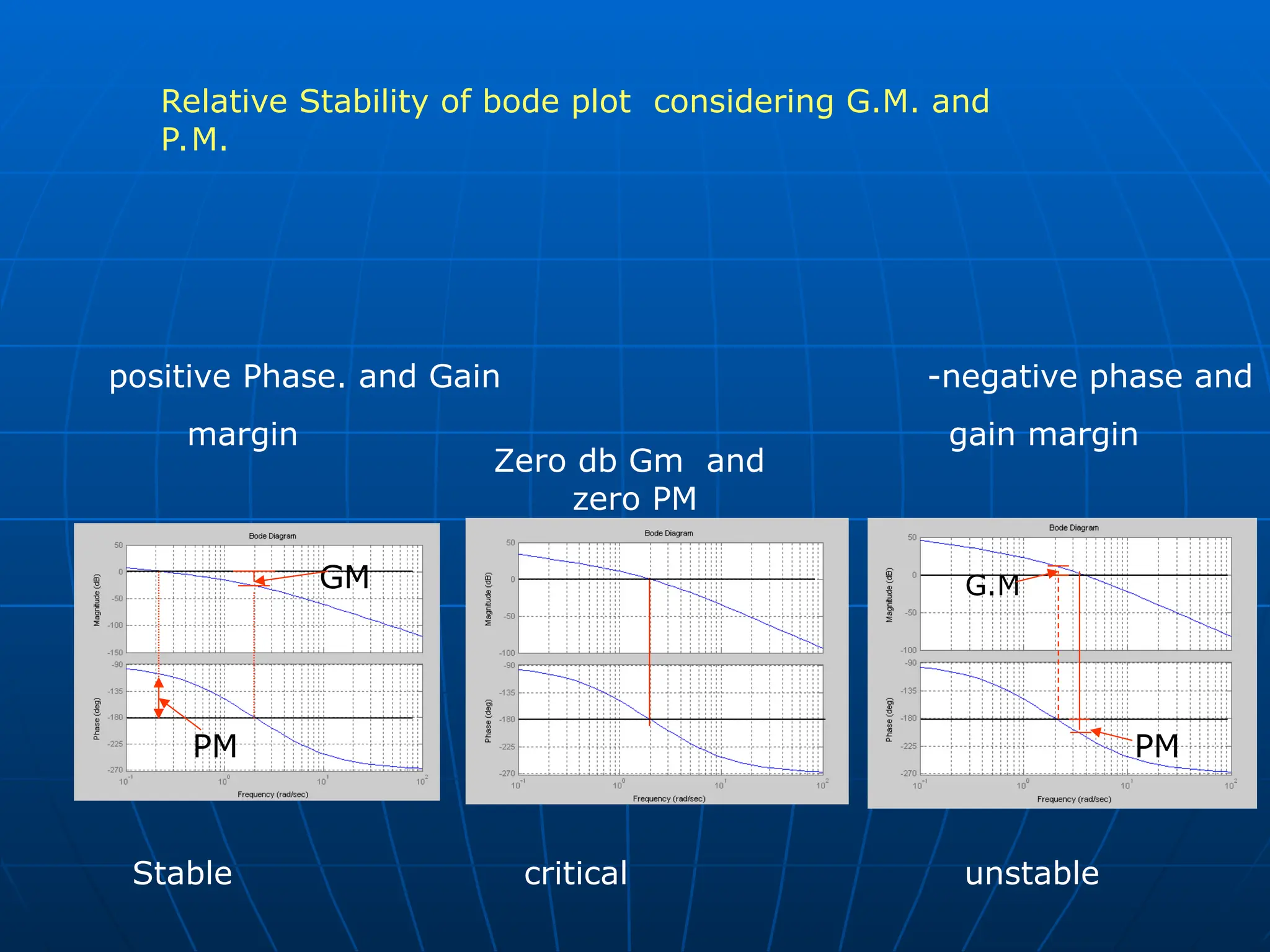
11. Gain and phase margin
Phase cross over
Gain cross over
gc
gain margin (GM) is defined as the
change in open loop gain required to
make the system unstable.
GM=-20log Ap at phase =-180o
phase margin (PM) is defined as the
change in open loop phase shift required
to make a closed loop system unstable.
at unity amplitude
180
)
( 1 

 
P
A
PM 


MATLAB Commands
Num=[ ];
Den=[ ];
Sys=tf(num,den);
[ gm pm gc pc]=Margin(sys)

12. Relative Stability of bode plot considering G.M. and
P.M.
Stable critical unstable
positive Phase. and Gain -negative phase and
margin gain margin
G.M
PM
GM
PM
Zero db Gm and
zero PM

13. Summary
current sequence covered stability analysis of control system using
current sequence covered stability analysis of control system using
Bode plot
Bode plot
Phase margin and gain margin
Phase margin and gain margin
With MATLAB application
With MATLAB application

14. Assessment
Assessment
To view the assessment click on the
To view the assessment click on the
link below.
link below.
Good Luck
Good Luck