The document discusses image segmentation techniques. It defines image segmentation as partitioning a digital image into multiple segments or regions that are similar in characteristics such as color or texture. The main goal of image segmentation is to simplify an image into meaningful parts for analysis. Common techniques discussed include thresholding, clustering, edge detection, region growing, and neural networks. Thresholding uses threshold values to separate pixels into multiple classes or objects. Clustering groups similar image pixels together while edge detection finds boundaries between objects. The document also provides an example of the split and merge segmentation method.

1. Unit 3 1
1) What do you mean by Image Segmentation?
Digital image processing is the use of computer algorithms to perform image processing into digital
images.Image segmentation is very important and challenging process of image processing. Image
segmentation is the techniques are used to partition an image into meaningful parts have similar
features and properties.
The aim of segmentation is simplification i.e. representing an image into meaningful and easily
analyzable way. Image segmentation is the first step in image analysis. The main goal of image
segmentation is to divide an image into several parts/segments having similar features or attributes.
The main applications of image segmentation are: Medical imaging, Content-based image
retrieval, Automatic traffic control systems, Object detection and Recognition Tasks, etc.
The image segmentation can be classified into two basic types: ​
Local segmentation (concerned with specific part or region of image) and ​
Global segmentation​ (concerned with segmenting in whole image, consisting of large number of
pixels).
11) Define segmentation. State different methods based on similarity.Explain any one
method with example.
Refer Q1.and Q5.
28) What is an ‘edge’ in an image? On what mathematical operation are the two
basic approaches for edge detection based on?
Refer Q6.
2)Explain the classification of image segmentation techniques.
Categories of Image Segmentation Methods
Clustering Methods- Level Set Methods
Histogram-Based Method- Graph portioning methods
Edge Detection Methods- Watershed Transformation
Region Growing Methods -Neural Networks Segmentation
3)Explain clustering technique used for image segmentation.
Defined as the process of identifying groups of similar image primitive.
It is a process of organizing the objects into groups based on its attributes.
An image can be grouped based on keyword (metadata) or its content (description)
KEYWORD- Form of font which describes about the image keyword of an image refers to its different
features
CONTENT- Refers to shapes, textures or any other information that can be inherited from the image
itself.
An image analysis is a process to extract some useful and meaningful information from an image.
Segmentation is one of the methods used for image analyses. Image segmentation has many
techniques to extract information from an image. Clustering is a technique which is used for image
segmentation. The main goal of clustering is to differentiate the objects in an image using similarity

2. Unit 3 2
and dissimilarity between the regions. K-Nearest Neighbour is a classification method. K-mean is a
clustering technique which is a simple and an iterative method.
21.Name different types of image segmentation techniques. Explain the
splitting and merging technique with the help of example.
18. Write a short note on region splitting
Region Splitting
i. The basic idea of region splitting is to break the image into a set of disjoint regions,
ii. which are coherent within themselves:
iii. Initially take the image as a whole to be the area of interest.
iv. Look at the area of interest and decide if all pixels contained in the region satisfy some
v. similarity constraint.
vi. If TRUE then the area of interest corresponds to an entire region in the image.
vii. If FALSE split the area of interest (usually into four equal subareas) and consider each of the
sub-areas as the area of interest in turn.
viii. This process continues until no further splitting occurs. In the worst case this happens when
the areas are just one pixel in size.
ix. If only a splitting schedule is used then the final segmentation would probably contain many
neighboring regions that have identical or similar properties.
x. We need to merge these regions
Region Merging
i. The result of region merging usually depends on the order in which regions are merged.
ii. The simplest methods begin merging by starting the segmentation using regions of 2x2, 4x4 or
8x8 pixels.
iii. Region descriptions are then based on their statistical gray levelproperties.
iv. A region description is compared with the description of an adjacent region; if they match, they
are merged into a larger region and a new region description is computed.
v. Otherwise regions are marked as non-matching.
vi. Merging of adjacent regions continues between all neighbors, including newly formed ones.
vii. If a region cannot be merged with any of its neighbors, it is marked `final' and the merging
process stops when all image regions are so marked.
Merging Heuristics:
Two adjacent regions are merged if a significant part of their common boundary consists of weak
edges
Two adjacent regions are also merged if a significant part of their common boundary consists of
weak edges, but in this case not considering the total length of the region borders.
Of the two given heuristics, the first is more general and the second cannot be used alone because it
does not consider the influence of different region sizes.
Region merging process could start by considering small segments (2*2,... ,8*8) selected a priori from
the image segments generated by thresholding regions generated by a region splitting module
The last case is called as “Split and Merge” method. Region merging methods generally use similar
criteria of homogeneity as region splitting methods, and only differ in the direction of their
application.
To illustrate the basic principle of split and merge methods, let us consider an imaginary image.

3. Unit 3 3
Let I denote the whole image shown in Fig. (a)
Not all the pixels in Fig (a) are similar. So the region is split as in Fig. (b).
Assume that all pixels within each of the regions I1, I2 and I3 are similar, but those in I4 are not.
Therefore I4 is split next, as shown in Fig. (c).
Now assume that all pixels within each region are similar with respect to that region, and that after
comparing the split regions, regions I43 and I44 are found to be identical.
i. A combination of splitting and merging may result in a method with the advantages of both the
approaches.
ii. Split-and-merge approaches work using pyramid image representations.
iii. Regions are square-shaped and correspond to elements of the appropriate pyramid level.
iv. If any region in any pyramid level is not homogeneous (excluding the lowest level). it is split into
four sub-regions -- these are elements of higher resolution at the level below.
v. If four regions exist at any pyramid level with approximately the same value of homogeneity
measure.
vi. They are merged into a single region in an upper pyramid level.
vii. We can also describe the splitting of the image using a tree structure, called a modified quadtree.
viii.Each non-terminal node in the tree has at most four descendants, although it may have less due to
merging.
ix. Quadtree decomposition is an operation that subdivides an image into blocks that contain
"similar" pixels.
x. Usually the blocks are square, although sometimes they may be rectangular.
xi. For the purpose of this demo, pixels in a block are said to be"similar" if the range of pixel values in
the block are not greater than some threshold.
xii. Quadtree decomposition is used in variety of image analysis and compression applications.
xiii.An unpleasant drawback of segmentation quadtrees, is the square region shape assumption.
xiv. It is not possible to merge regions which are not part of the same branch of the segmentation tree.
xv. Because both split-and-merge processing options are available,the starting segmentation does not
have to satisfy any of the homogeneity conditions.
xvi. The segmentation process can be understood as the construction of a segmentation quadtree
where each leaf node represents a homogeneous region.
xvii. Splitting and merging corresponds to removing or building parts of the segmentation quadtree
Split& Merge

4. Unit 3 4
4)How is thresholding used in image segmentation?
Thresholding is one of the most important techniques for segmentation and because of its simplicity,
is widely used. In segmentation, thresholding is used to produce regions of uniformity within the
given image based on some threshold criteria T.
Suppose, we have an image which is compared of dark objects of varying grey levels against a light
background of varying grey levels.
There are 2 types of thresholding:
1. Global Thresholding.
2. Local Thresholding
Global Thresholding: ​
Global Thresholding​ . A histogram of the input image intensity should reveal two peaks,
corresponding respectively to the signals from the background and the object. ​
Global thresholding​ is as good as the degree of intensity separation between the two peaks in the
image. It is an unsophisticated segmentation choice.
Local Thresholding: In local adaptive technique, a threshold is calculated for each pixel, based on
some local statistics such as range, variance, or surface-fitting parameters of the neighborhood pixels.
Itcan be approached in different ways such as background subtraction, water flow model, means and
standard derivation of pixel values, and local image contrast.

5. Unit 3 5
29)Give the following kernel:
Prewitt:
The Prewitt edge detection is proposed by Prewitt in 1970 (Rafael C.Gonzalez
To estimatethe magnitude and orientation of an edge Prewitt is a correct way.
Even though different gradient edge detection wants a quite time consuming calculation to estimate
the direction from the magnitudes in the x and y-directions, the compass edge detection obtains the
direction directly from the kernel with the highest response.
It is limited to 8 possible directions; however knowledge shows that most direct direction estimates
are not much more perfect. This gradient based edge detector is estimated in the 3x3 neighborhood
for eight directions.
All the eight convolution masks are calculated. One complication mask is then selected, namely with
the purpose of the largest module.
2.Robert:
The ​ Roberts cross​ operator is used in image processing and computer vision for edge
detection. It was one of the first edge detectors and was initially proposed by Lawrence Roberts in
1963. As a differential operator, the idea behind the Roberts cross operator is to approximate the
gradient of an image through discrete differentiation which is achieved by computing the sum of
the squares of the differences between diagonally adjacent pixels.
2)Sobel:
The Sobel edge detection method is introduced by Sobel in 1970 (Rafael C.Gonzalez (2004)).
The Sobel method of edge detection for image segmentation finds edges using the Sobel
approximation to the derivative.
It precedes the edges at those points where the gradient is highest.
The Sobel technique performs a 2-D spatial gradient quantity on an image and so highlights regions of
high spatial frequency that correspond to edges.
In general it is used to find the estimated absolute gradient magnitude at each point in n input
grayscale image.
Inconjecture at least the operator consists of a pair of 3x3 complication kernels as given away in under
table. One kernel is simply the other rotated by 90degree.
This is very alike to the Roberts Cross operator.
-1 -2 -1
0 0 0
1 2 1
Gx Gy
-1 0 -1
-2 0 2
-1 0 1

6. Unit 3 6
6) Explain various edges detected in segmentation process.
Edge detection is a process of locating an edge of an image. Detection of edges in an
image is avery important step towards understanding image features. Edges consist of
meaningful features and contained significant information. It reduces significantly the
amount of the image size and filters out information that may be regarded as less
relevant, preserving the important structural properties of an image.
There are many methods of detecting edges; the majority of different methods may be
grouped into these two categories:
Gradient: The gradient method detects the edges by looking for the maximum and
minimum in the first derivative of the image. For example Roberts, Prewitt, Sobel
operators detect vertical and horizontal edges. Sharp edges can be separated out by
appropriate thresholding.
Laplacian: The Laplacian method searches for zero crossings in the second derivative
of the image to find edges e.g. Marr-Hildreth, Laplacian of Gaussian etc.
Explain gradient operator and laplacian operator.
The gradient of the image is one of the fundamental building blocks in image processing.
The most common way to approximate the image gradient is to convolve an image with
a kernel, such as the Sobel operator or Prewitt operator.

7. Unit 3 7
Laplacian Operator is also a derivative operator which is used to find edges in an image.
The major difference between Laplacian and other operators like Prewitt, Sobel,
Robinson and Kirsch is that these all are first order derivative masks but Laplacian is a
second order derivative mask. In this mask we have two further classifications one is
Positive Laplacian Operator and other is Negative Laplacian Operator.
In Positive Laplacian we have standard mask in which center element of the mask
should be negative and corner elements of mask should be zero.
Positive Laplacian Operator is use to take out outward edges in an image.
0 1 0
1 -4 1
0 1 0
Negative Laplacian Operator
In negative Laplacian operator we also have a standard mask, in which center element
should be positive. All the elements in the corner should be zero and rest of all the
elements in the mask should be -1.
0 -1 0

8. Unit 3 8
-1 4 -1
0 -1 0
Negative Laplacian operator is use to take out inward edges in an image
31) Write a short note on Laplacian of Gaussian (LOG).
Laplacian filters are derivative filters used to find areas of rapid change (edges) in
images. Since derivative filters are very sensitive to noise, it is common to smooth the
image (e.g., using a Gaussian filter) before applying the Laplacian.
Wherever a change occurs, the LoG will give a positive response on the darker side and
a negative response on the lighter side. At a sharp edge between two regions, the
response will be
1. zero away from the edge
2. positive just to one side
3. negative just to the other side
4. zero at some point in between on the edge itself
When using the filter given above, or any other similar filter, the output can contain
values that are quite large and may be negative, so it is important to use an image type
that supports negatives and a large range, and then scale the output.
32) Explain the term Difference of Gaussians Filter (DoG).
The Difference of Gaussian module is a filter that identifies edges. The DOG filter is
similar to the LOG(Laplacian of Gaussian) and DOB(Difference Of Box) filters in that
it is a two stage edge detection process.
The DOG performs edge detection by performing a Gaussian blur on an image at a
specified theta (also known as sigma or standard deviation). The resulting image is a
blurred version of the source image. The module then performs another blur with a
sharper theta that blurs the image less than previously. The final image is then
calculated by replacing each pixel with the difference between the two blurred images
and detecting when the values cross zero, i.e. negative becomes positive and vice versa.
The resulting zero crossings will be focused at edges or areas of pixels that have some
variation in their surrounding neighborhood.

9. Unit 3 9
9) ​ What is edge linking? Highlight its significance in image segmentation.
Edge detectors yield pixels in an image lie on edges.
The next step is to try to collect these pixels together into a set of edges.
Thus, our aim is to replace many points on edges with a few edges themselves.
The practical problem may be much more difficult than the idealised case.
● Small pieces of edges may be missing,
● Small edge segments may appear to be present due to noise where there is no
real edge, ​ etc​ .
In general, edge linking methods can be classified into two categories:
Local Edge Linkers
where edge points are grouped to form edges by considering each point's relationship
to any neighbouring edge points.
Global Edge Linkers
where all edge points in the image plane are considered at the same time and sets of
edge points are sought according to some similarity constraint, such as points which
share the same edge equation.
15) Explain the method of edge linking using Hough transform.
Hough transform can be used for pixel linking and curve detection.
Line detection using Hough transform:
Map all the edge points from xy plane to ab plane using Hough Transform.
Eg: Consider a edge points in
A​ (​ x​ 1,​ ​ y​ 1),​ ​ B​ (​ x​ 2,​ ​ y​ 2),​ ​ C​ (​ x​ 3,​ ​ y​ 3)​ ​ and
D​ (​ x​ 4,​ ​ y​ 4)​
as shown in below figure.

10. Unit 3 10
Count the number of intersecting lines at each point in ab plane
Select the point with maximum value of count.
Eg: Max value of count is 3 at point (a’,b’)
Define line with slope value =a’ and y constant value=b’
The equation of line is y’=a’x+b’
Determine co-linear points
Eg:pt A, B, C are co-linear pts
Link Co-linear points
Limitations of the Hough transform:
This algorithm is not suitable for vertical lines where slope=∞ m= =∞

11. 11
COMPRESSION
4) Compare and contrast between inter pixel redundancy, coding redundancy and psycho-
visual redundancy.
Redundancy can be broadly classified into Statistical redundancy and Psycho visual redundancy.
Statistical redundancy can be classified into inter-pixel redundancy and coding redundancy.
Inter-pixel can be further classified
Coding Redundancy:
● Coding redundancy is associated with the representation of information.
● The information is represented in the form of codes.
● If the gray levels of an image are coded in a way that uses more code symbols than absolutely
necessary to represent each gray level then the resulting image is said to contain coding
redundancy.
Inter-pixel Spatial Redundancy:
● Interpixel redundancy is due to the correlation between the neighboring pixels in an image.
● That means neighboring pixels are not statistically independent. The gray levels are not
equally probable.
Inter-pixel Temporal Redundancy:
● Interpixel temporal redundancy is the statistical correlation between pixels from successive
frames in video sequence.
● Temporal redundancy is also called interframe redundancy. Temporal redundancy can
be exploited using motion compensated predictive coding.
Psychovisual Redundancy:
● The Psychovisual redundancies exist because human perception does not involve
quantitative analysis of every pixel or luminance value in the image.
● It’s elimination is real visual information is possible only because the information itself is not
essential for normal visual processing.
into spatial redundancy and temporal redundancy.

12. 12
7) Explain Huffman coding with suitable example.
Huffman coding algorithm was invented by David Huffman in 1952. It is an algorithm
which works with integer length codes. A Huffman tree represents Huffman codes for
the character that might appear in a text file. Unlike to ASCII or Unicode, Huffman
code uses different number of bits to encode letters. If the number of occurrence of any
character is more, we use fewer numbers of bits. Huffman coding is a method for the
construction of minimum redundancy codes.
Huffman tree can be achieved by using compression technique. Data compression have
lot of advantages such as it minimizes cost, time, bandwidth, storage space for
transmitting data from one place to another.
Huffman Coding Algorithm Example:

13. 13

14. 14
10) Explain the JPEG compression with suitable block diagram.
JPEG​ is a commonly used method of lossy compression for digital images,
particularly for those images produced by digital photography. The degree of
compression can be adjusted, allowing a selectable tradeoff between storage size and
image quality.
JPEG uses a lossy form of compression based on the discrete cosine transform (DCT).
This mathematical operation converts each frame/field of the video source from the
spatial (2D) domain into the frequency domain (a.k.a. transform domain). A
perceptual model based loosely on the human psychovisual system discards high-
frequency information, i.e. sharp transitions in intensity, and color hue. In the
transform domain, the process of reducing information is called quantization. In
simpler terms, quantization is a method for optimally reducing a large number scale
(with different occurrences of each number) into a smaller one, and the transform-
domain is a convenient representation of the image because the high-frequency
coefficients, which contribute less to the overall picture than other coefficients, are
characteristically small-values with high compressibility.
The compression method is usually lossy, meaning that some original image
information is lost and cannot be restored, possibly affecting image quality. There is
an optional lossless mode defined in the JPEG standard. However, this mode is not
widely supported in products.
The digital wavelets transform (DWT) converts a large portion of the original image to
horizontal, vertical and diagonal decomposition coefficients with zero mean and
Laplacianlike distributions.
Many computed coefficients can be quantized and coded to minimize Interco
efficient and coding redundancy.
The quantization can be adapted to exploit any positional correlation across
different decomposition levels.
Subdivision of the original image is unnecessary :
Eliminating the blocking artifact that characterizes DCT-based approximations at
high compression ratios.

15. 15
13) Compare arithmetic coding and Huffman coding.
Huffman Coding vs.Arithmetic Coding: Huffman Coding Algorithm uses a static table
for the whole coding process, so it is faster.
However it does not produce efficient compression ratio.On the contrary,
Arithmetic algorithm can generate a high compression ratio, but its compression
speed is slow. The table presents a simple comparison between these compression
methods.

16. 16
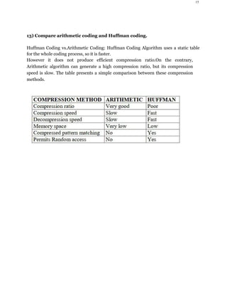
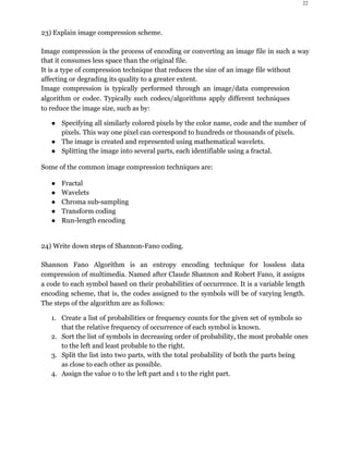
12) Block Diagram of JPEG encoder and Decoder.
1) Forward Discrete Cosine Transform (FDCT):
The still images are first partitioned into non-overlapping blocks of size 8x8 and the
image samples are shifted from unsigned integers with range [0, 2 p-1] to signed
integers
with range [-2 p-1, 2 p-1], where p is the number of bits (here,p=8 ).
To preserve freedom for innovation and customization within implementations, JPEG
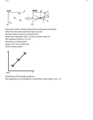
neither specifies any unique FDCT algorithm, nor any unique IDCT algorithms.
2) Quantization:
Each of the 64 coefficients from the FDCT outputs of a block is uniformly quantized
according to a quantization table.
Since the aim is to compress the images without visible artifacts, each step-size
should be chosen as the perceptual threshold or for “just noticeable distortion”.
The quantized coefficients are zig-zag scanned.
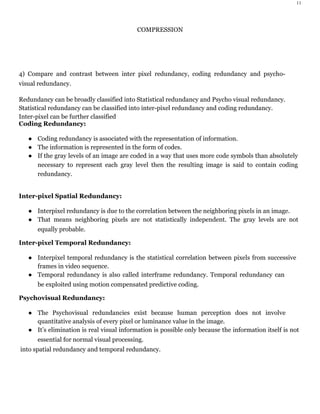
The DC coefficient is encoded as a difference from the DC coefficient of the previous
block and the 63 AC coefficients are encoded into (run, level) pair.
3) Entropy Coder:
This is the final processing step of the JPEG encoder.
The JPEG standard specifies two entropy coding methods – Huffman and arithmetic
coding.
The baseline sequential JPEG uses Huffman only, but codecs with both methods are
specified for the other modes of operation.
Huffman coding requires that one or more sets of coding tables are specified by the
application.
The same table used for compression is used needed to decompress it.
The baseline JPEG uses only two sets of Huffman tables – one for DC and the other
for AC.

17. 17
14) Explain with block diagram Transform based coding.
Transform coding is used to convert spatial image pixel values to transform
coefficient values. Since this is a linear process and no information is lost, the
number of coefficients produced is equal to the number of pixels transformed.
The desired effect is that most of the energy in the image will be contained in a few
large transform coefficients. If it is generally the same few coefficients that contain
most of the energy in most pictures, then the coefficients may be further coded by
lossless entropy coding . In addition, it is likely that the smaller coefficients can be
coarsely quantized or deleted ( lossy coding ) without doing visible damage to the
reproduced image.
Many types of transforms have been tried for picture coding, including for example
Fourier, Karhonen-Loeve, Walsh-Hadamard, lapped orthogonal, discrete cosine

18. 18
(DCT), and recently, wavelets. The various transforms differ among themselves in
three basic ways that are of interest in picture coding:
1) the degree of concentration of energy in a few coefficients;
2) the region of influence of each coefficient in the reconstructed picture;
3) the appearance and visibility of coding noise due to coarse quantization of
the coefficients.
16) What are different types of data redundancies found in a digital
image? Explain in detail.
Image compression is possible because images, in general are highly coherent, which
means that there is redundant information. Compression is achieved through
redundancy and irrelevancy reduction. Redundancy can be broadly classified into:
(i) Statistical Redundancy (ii) Psychovisual Redundancy
Statistical Redundancy:​ As stated, statistical redundancy can be classified
into two types:
(i) Interpixel redundancy (ii) Coding redundancy.
Interpixel redundancy is due to the correlation between neighbouring pixels in an
image. It means that the neighbouring pixels are not statically independent. The
interpixel correlation is referred as interpixel redundancy. Coding redundancy is
associated with the representation of
information. The information is represented in the form of codes. The Huffman code
and arithmetic codes are some examples of codes.
Psychovisual redundancy:​ Psychovisual redundancy is associated with the
characteristics of the human visual system (HVS). In the HVS, visual information is
not perceived equally. Some information may be more important than other
information. If less data is used to represent less important visual information,
perception will not be affected. This implies that visual information is psychovisually
redundant Eliminating the psychovisual redundancy leads to efficient compression.
Spatial Redundancy:​ Spatial redundancy represents the statistical correlation
between neighbouring pixels in an image. It is not necessary to represent implies that
there is a relationship between neighbouring pixels in an image. It is not necessary to
represent each pixel in an image independently. Instead a pixel is predicted from its
neighbours. Removing spatial redundancy through prediction is basic principle of
differential coding which is widely employed in image and video compression.
Temporal Redundancy:​ Temporal redundancy is the statistical correlation
between pixels from successive frames in a video sequence. The temporal
redundancy is also called interframe redundancy. Motion compensated predictive
coding is employed to reduce temporal redundancy. Removing a large amount of
temporal redundancy leads to efficient video compression.

19. 19
17) Generate the Huffman code for the word ‘COMMITTEE’.
Total number of symbols in the word COMMITTEE is 9.
Probability of a symbol C = p(C)= 1/9
Probability of a symbol O= p(O)=1/9
Probability of a symbol M=p(M)=2/9
Probability of a symbol I=p(I)= 1/9
Probability of a symbol T=p(T)= 2/9
Probability of a symbol E=p(E) =2/9

20. 20
19) Explain run length coding with suitable example.
Run-length encoding​ (​ RLE​ ) is a very simple form of lossless data
compression in which ​ runs​ of data (that is, sequences in which the same data value
occurs in many consecutive data elements) are stored as a single data value and count,
rather than as the original run.
This is most useful on data that contains many such runs. Consider, for example,
simple graphic images such as icons, line drawings, Conway’s Game of Life, and
animations.
It is not useful with files that don't have many runs as it could greatly increase the file
size.
RLE may also be used to refer to an early graphics file format supported by
CompuServe for compressing black and white images, but was widely supplanted by
their later Graphics Interchange Format.
RLE also refers to a little-used image format in Windows 3.x, with the extension
​ rle​ , which is a Run Length Encoded Bitmap, used to compress the Windows 3.x
startup screen.
i. In one-dimensional run-length coding schemes for binary images, runs of
continuous 1’s or 0’s in every row of an image are encoded together, resulting
insubstantial bit savings.
ii. Either, it is to be indicated whether the row begins with a run of 1s or 0s.
iii. Run-length encoding may be illustrated with the following example of a row of an
image:
000110100011111
iv. The first run count in the given binary sequence is 0.
v. Then we have a run of three 0s.
vi. Hence, the next count is 3.
vii. Proceeding in this manner, the reader may verify that the given binary sequence
gets encoded to: 0,3,2,1,1,3,5
viii. Can compress any type of data but cannot achieve high compression ratios
compared to other compression methods.

21. 21
22) Compare lossy and lossless image compression.

22. 22
23) Explain image compression scheme.
Image compression is the process of encoding or converting an image file in such a way
that it consumes less space than the original file.
It is a type of compression technique that reduces the size of an image file without
affecting or degrading its quality to a greater extent.
Image compression is typically performed through an image/data compression
algorithm or codec. Typically such codecs/algorithms apply different techniques
to reduce the image size, such as by:
● Specifying all similarly colored pixels by the color name, code and the number of
pixels. This way one pixel can correspond to hundreds or thousands of pixels.
● The image is created and represented using mathematical wavelets.
● Splitting the image into several parts, each identifiable using a fractal.
Some of the common image compression techniques are:
● Fractal
● Wavelets
● Chroma sub-sampling
● Transform coding
● Run-length encoding
24) Write down steps of Shannon-Fano coding.
Shannon Fano Algorithm is an entropy encoding technique for lossless data
compression of multimedia. Named after Claude Shannon and Robert Fano, it assigns
a code to each symbol based on their probabilities of occurrence. It is a variable length
encoding scheme, that is, the codes assigned to the symbols will be of varying length.
The steps of the algorithm are as follows:
1. Create a list of probabilities or frequency counts for the given set of symbols so
that the relative frequency of occurrence of each symbol is known.
2. Sort the list of symbols in decreasing order of probability, the most probable ones
to the left and least probable to the right.
3. Split the list into two parts, with the total probability of both the parts being
as close to each other as possible.
4. Assign the value 0 to the left part and 1 to the right part.

23. 23
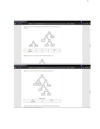
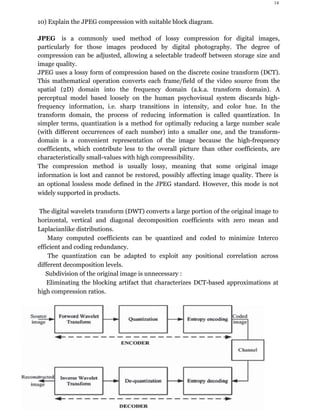
5. Repeat the steps 3 and 4 for each part, until all the symbols are split into
individual subgroups.
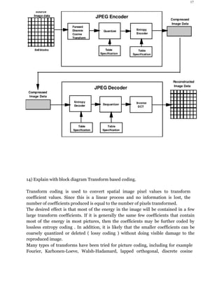
25)How Arithmetic coding is used in image compression?
Arithmetic coding is a common algorithm used in both lossless and lossy data
compression algorithms.
It is an entropy encoding technique, in which the frequently seen symbols are encoded
with fewer bits than rarely seen symbols. It has some advantages over well-known
techniques such as Huffman coding.
The first thing to understand about arithmetic coding is what it produces.
Arithmetic coding takes a message (often a file) composed of symbols (nearly always
eight-bit characters), and converts it to a floating point number greater than or equal to
zero and less than one.
This floating point number can be quite long - effectively your entire output file is one
long number - which means it is not a normal data type that you are used to using in
conventional programming languages.
The implementation of the algorithm will have to create this floating point number
from scratch, bit by bit, and likewise read it in and decode it bit by bit.
This encoding process is done incrementally. As each character in a file is encoded, a
few bits will be added to the encoded message, so it is built up over time as the
algorithm proceeds.
The second thing to understand about arithmetic coding is that it relies on a model​ to
characterize the symbols it is processing. The job of the model is to tell the encoder
what the probability of a character is in a given message.
If the model gives an accurate probability of the characters in the message, they will be
encoded very close to optimally. If the model misrepresents the probabilities of symbols,
your encoder may actually expand a message instead of compressing it.
Arithmetic coding solves many limitations of Huffman coding.
i. Arithmetic encoders are better suited for adaptive models than Huffman coding.
ii. It is an entropy encoding technique, in which the frequently seen symbols are
encoded with fewer bits than lesser seen symbols.
iii. No assumption on encode source symbols one at a time.
iv. Sequences of source symbols are encoded together.
v. There is no one-to-one correspondence between source symbols and code words.
vi. Slower than Huffman coding but typically achieves better compression.
vii. A sequence of source symbols is assigned a single arithmetic code word which
corresponds to a sub-interval in [0,1].
viii. As the number of symbols in the message increases, the interval used to
represent it becomes smaller.
ix. Smaller intervals require more information units (i.e., bits) to be represented.

24. 24
26) Explain image compression standards.
Most of the standards are issued by
International Standardization Organization (ISO)
Consultative Committee of the International Telephone and Telegraph (CCITT)
CCITT Group 3 and 4 are for binary image compression
Originally designed as fasimile(FAX) coding method
G3 : Nonadaptive, 1-D run-length coding
G4 : a simplified or streamlined version of G3, only 2-D coding
The coding approach is quite similar to the RAC method
Joint BilevelImaging Group (JBIG)
A joint committee of CCITT and ISO
Proposed JBIG1: adaptive arithmetic compression technique (the best average and
worst-case available)
Proposed JBIG2 : achieve compressions 2 to 4 times greater than JBIG1
27)What is block processing? Explain in detail.
***
28) Explain various JPEG modes.
The JPEG standard defined four compression modes: Hierarchical, Progressive,
Sequential and lossless.
Sequential​ : Sequential-mode images are encoded from top to bottom.
Sequential mode supports sample data with 8 and 12 bits of precision. In the
sequential JPEG, each color component is completely encoded in single scan.
Within sequential mode, two alternate entropy encoding processes are
defined by the JPEG standard: one uses Huffman encoding; the other uses
arithmetic coding.
2. Progressive​ : In progressive JPEG images, components are encoded in
multiple scans. The compressed data for each component is placed in a
minimum of 2 and as many as 896 scans. The initial scans create a rough version
of the image, while subsequent scans refine it.
3. Lossless​ : preserves exact, original image, small compression ration, less use
4. Hierarchical​ : JPEG is a super-progressive mode in which the image Is
broken down into a number of subimages called frames. A frame is a collection
of one or more scans. In hierarchical mode, the first frame creates a low-
resolution version of image. The remaining frames refine the image by increasing
the solution.

25. 25
29) What is content-based image retrieval?
Also known as Query By Image Content (QBIC), presents the technologies allowing to
organize digital pictures by their visual features. They are based on the application of
computer vision techniques to the image retrieval problem in large databases.
Content-Based Image Retrieval (CBIR) consists of retrieving the most visually similar
images to a given query image from a database of images.
A process framework for efficiently retrieving images from a collection by similarity.
The retrieval relies on extracting the appropriate characteristic quantities describing
the desired contents of images. In addition, suitable querying, matching, indexing and
searching techniques are required.
The field of representing, organising and searching images based on their content
rather than image annotations.
30) Explain Frei-Chen Edge Detector and give the nine masks.
Frei-Chen Edge Detector shows similarities to the Sobel Operator. It also works on a
3×3 texel footprint but applies a total of nine convolution masks to the image. Frei-
Chen masks are unique masks, which contain all of the basis vectors. This implies that a
3×3 image area is represented with the weighted sum of nine Frei-Chen masks that can
be seen below:
The first four Frei-Chen masks above are used for edges, the next four are used for
lines and the last mask is used to compute averages. For edge detection, appropriate
masks are chosen and the image is projected onto i

26. 26