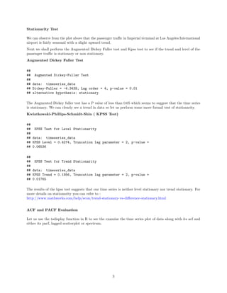
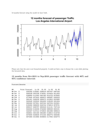
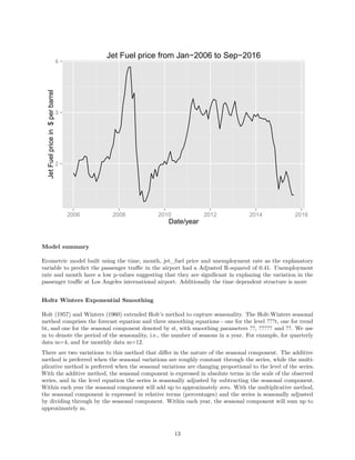
This document presents a comprehensive analysis of forecasting passenger traffic at Los Angeles International Airport, utilizing various models including ARIMA, econometric, and exponential smoothing techniques. It outlines the methodologies for data gathering, analysis, and the resulting forecasts for passenger activity from October 2015 to September 2016, highlighting the importance of accurately predicting air traffic for effective airport planning. The study emphasizes the significance of socio-economic variables and historical data trends in developing reliable forecasting models.

1. FORECASTING AVIATION ACTIVITY
Los Angeles International airport
Prepared by:
Rupantar Rana
MS Business Analytics Student
Marshall School of Business
University of Southern California
rupantar@marshall.usc.edu
December 2015

2. TABLE OF CONTENTS
Introduction and Motivation .......................................................................................
Data source identification and
description………………………………………………………………….
Initial Hypothesis……………………………………………………………………
Procedure 1: Arima Time series modelling…………………………………………
Step 1: Stationarity Test
Step 2: ACF and PACF plot Evaluation
Step 3: Candidate Model selection
Step 4: Residual Diagnosis
Step 5: 12 month Forecast with Confidence Interval
Procedure 2: Econometric Modelling
Step 1: Econometric Variable Identification
Step 2: Data Gathering
Step 3: Data Cleaning and Integration
Step 4: Model building and Model Selection
Step 5: Cross Validation
Procedure 3: Exponential Smoothing
Holt Winters Technique
Procedure 4: Ensemble Modelling
Average Ensemble Model
Apply Forecast Methods and Evaluate Results ...........................................................
Executive Summary document ……………………………………………………...

3. Time series analysis project
Rupantar Rana
Los Angeles International Airport - Passenger Traffic Prediction
Introduction and Motivation
Air traffic forecast serves as an important quantitative basis for airport planning - in particular for capacity
planning, CAPEX as well as for aeronautical and non-aeronautical revenue planning. High level decision and
planning in airports relies heavily on future airport activity. Many research have shown that airport traffic is
subject to great volatility now then has been the case in the past. Many past predictive models for air traffic
models have mixed performance due to unanticipated events and circumstances in the forcasts.
The goal of this analysis is to provide a realistic forecast based on latest available data to reflect the current
conditions at the airport, supported by information in the study providing an adequate justification for the
airport planning and development.
The aim here is to develop a model that can accurately predict the volume of air traffic in Los Angeles
International Airport using the dataset that is available from the data.gov website.
Data Description
Date Range : From 1/1/2006 to 9/1/2015
Datasource Description : The dataset contains details of the Passenger Traffic in Los Angeles International
Airport. It is a non-federal data set downloaded from the data.gov website. This dataset consists of 4286
rows and 9 columns and contains the following variables.
Data extraction date : This is the exact date at which the data was extracted. At this stage we can ignore
this variable as it is not related to the analysis.
Report Period : This is the date variable that is used as the date variable for the time series analysis.
Terminal : The airport terminal from Terninal 1 to Terminal 8 , Misc. Terminal and Tom Bradley
international airport.
Arrival Departure : This variable is used to indicate whether the passengers were recorded on arrival or
on departure.
Domestic International Airport : This variable indicates Whether it is a domestic or international airport
Passenger Count : The number of passengers recorded on that particular day.
https://catalog.data.gov/dataset/los-angeles-international-airport-passenger-traffic-by-terminal-756ee
Initial Hypothesis
From the research on passenger activity on airport, passenger traffic should have a time dependent structure.
Additionally, socio-economic factors could be used to explain some of the causal relationship with passenger
traffic. Air traffic activity could also be affected by interaction of supply and demand factors. The demand in
aviation is largely a function of demographic and economic factors. Supply factors such as cost, competition
and regulations could also help determine air traffic activity.
1

4. Aviation forecasting background and techniques
Some of the forecasting techniques that have been traditionally used include the following:
Time Series Forecasting : Time series trend and seasonality extrapolation using statistical techniques
that rely on past data to predict the future values
Econometric modelling with explanatory variables : This type of modelling techniques relies on
examining the relationship between traffic data and possible explanatory variables such as GDP, disposable
income, price of fuel and so forth
Simulations : A method where snapshots or samples of data can be regenerated using complex models to
explore and forecast the future values
Ensemble Modelling : Here the forecast of all the above mentioned methods can be combined to devise a
model that performs better than the individual methods
Market share analysis : A technique used to forecast a local activity as a share of a larger some larger
aggregated activity. eg. airport traffic may be based on national traffic which may have been forecasted by a
third party.
For our analysis we will be using time series analysis to model the time dependent structure of passenger
traffic behaviour for Los Angeles international Airport.
Procedure 1 : Time Series Analysis
We shall start by performing exploratory data analysis for the data set, then we shall investivate and come
up with candidate models for forecasting. We will use the best possible model to predict passenger activity.
Finally we will predict for the next 12 months from Oct-2015 to Sep-2016 with 80% and 95% confidence
intervals.
4e+06
5e+06
6e+06
7e+06
2006 2008 2010 2012 2014 2016
Date/year
PassengerCount
Passenger traffic: Los Angeles Internation Airport
2

5. Stationarity Test
We can observe from the plot above that the passenger traffic in Imperial terminal at Los Angeles International
airport is fairly seasonal with a slight upward trend.
Next we shall perform the Augmented Dickey Fuller test and Kpss test to see if the trend and level of the
passenger traffic is stationary or non stationary.
Augmented Dickey Fuller Test
##
## Augmented Dickey-Fuller Test
##
## data: timeseries_data
## Dickey-Fuller = -4.3439, Lag order = 4, p-value = 0.01
## alternative hypothesis: stationary
The Augmented Dickey fuller test has a P value of less than 0.05 which seems to suggest that the time series
is stationary. We can clearly see a trend in data so let us perform some more formal test of stationarity.
Kwiatkowski-Phillips-Schmidt-Shin ( KPSS Test)
##
## KPSS Test for Level Stationarity
##
## data: timeseries_data
## KPSS Level = 0.4274, Truncation lag parameter = 2, p-value =
## 0.06536
##
## KPSS Test for Trend Stationarity
##
## data: timeseries_data
## KPSS Trend = 0.1956, Truncation lag parameter = 2, p-value =
## 0.01765
The results of the kpss test suggests that our time series is neither level stationary nor trend stationary. For
more details on stationarity you can refer to :
http://www.mathworks.com/help/econ/trend-stationary-vs-difference-stationary.html
ACF and PACF Evaluation
Let us use the tsdisplay function in R to see the examine the time series plot of data along with its acf and
either its pacf, lagged scatterplot or spectrum.
3

6. Time series display output with ACF and PACF
2 4 6 8
4000000
0 10 20 30 40 50
−0.40.00.4
Lag
ACF
0 10 20 30 40 50
−0.40.00.4
Lag
PACF
As we can see from the above ACF curve there is significant seasonal lags. To incorporate these seasonal lags
in our model we need to perform seasonal differencing.
4

7. Lag 1 Seasonal Differenced:
Time series display output with ACF and PACF
2 3 4 5 6 7 8 9
−6e+054e+05
0 10 20 30 40 50
−0.20.20.6
Lag
ACF
0 10 20 30 40 50
−0.20.20.6
Lag
PACF
After removing the seasonal lags we can notice high auto correlation evident from the trend present in the
data. We need to perform further lag 1 differencing in order to make this data stationary.
5

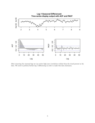
8. Double differenced data:
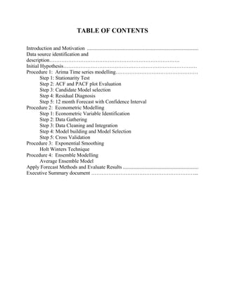
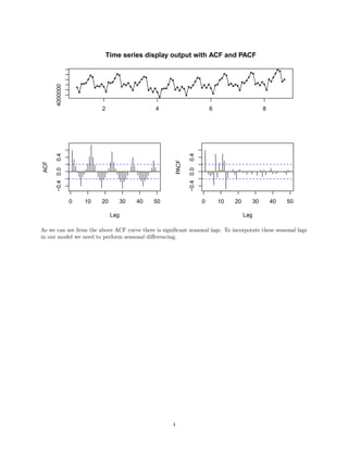
Time series display output with ACF and PACF
2 3 4 5 6 7 8 9
−3e+053e+05
0 10 20 30 40 50
−0.40.0
Lag
ACF
0 10 20 30 40 50
−0.40.0
Lag
PACF
Model Building
The ACF and PACF of the double differenced data suggests that the following ARIMA model could be the
best candidates :
ARIMA(0,1,1)[0,1,1][12]
We have now built the model and need to perform residual diagnosis before we move on to predict using the
model.
6

9. Residual Diagnosis
Residual Diagnosis of our model
2 4 6 8
−3e+053e+05
0 5 10 15 20 25 30
−0.30.00.2
Lag
ACF
0 5 10 15 20 25 30
−0.30.00.2
Lag
PACF
The residuals seem fairly linear in distribution and they do not show any significant auto correlation which
means that our model is adequately built. Let us further examine the residuals for test of significant
autocorrelation by examining performing the Box test.
##
## Box-Pierce test
##
## data: residuals_Model_Imperial_Terminal_1
## X-squared = 0.1366, df = 1, p-value = 0.7117
The P-value of the Box test is high suggesting that the residuals are not auto correlated.
Let us go ahead and forecast with our model.
7

10. Histogram of model Residuals
Residuals
Frequency
−4e+05 0e+00 4e+05
0102030
−2 −1 0 1 2−3e+05−1e+051e+053e+05
Normal Q−Q Plot
Theoretical Quantiles
SampleQuantiles
The standard assumption in linear regression is that the theoretical residuals are independent and normally
distributed. We can see from the above histogram and the qq plot, that the residuals confirm to this
assumption of normality.
8

11. 12 months forecast using the model we have built.
12 months forecast of passenger Traffic
Los Angeles International Airport
2 4 6 8 10
400000055000007000000
Please note that the axis is not formatted properly. I could not find a way to format the x axis while plotting
the forcasted data.
12 months from Oct-2015 to Sep-2016 passenger traffic forecast with 80% and
95% confidence intervals
Forecast12months
## Point Forecast Lo 80 Hi 80 Lo 95 Hi 95
## Nov 8 5262340 5128361 5396319 5057437 5467243
## Dec 8 5565038 5403786 5726291 5318424 5811653
## Jan 9 5296893 5112392 5481393 5014723 5579062
## Feb 9 4779445 4574420 4984470 4465887 5093003
## Mar 9 5661901 5438228 5885575 5319822 6003980
## Apr 9 5563426 5322543 5804308 5195028 5931824
## May 9 5830493 5573551 6087434 5437534 6223451
## Jun 9 6162690 5890635 6434744 5746619 6578761
## Jul 9 6569157 6282787 6855528 6131191 7007124
## Aug 9 6444343 6144339 6744348 5985526 6903161
## Sep 9 5420457 5107412 5733503 4941696 5899219
## Oct 9 5626821 5301256 5952385 5128913 6124728
## Nov 9 5373930 5026626 5721234 4842774 5905085
## Dec 9 5675364 5310894 6039834 5117955 6232773
9

12. ## Jan 10 5405630 5024709 5786551 4823062 5988198
## Feb 10 4890188 4493782 5286595 4283937 5496439
## Mar 10 5765533 5354224 6176842 5136491 6394576
## Apr 10 5672429 5246739 6098120 5021392 6323467
## May 10 5934131 5494530 6373733 5261819 6606444
## Jun 10 6263639 5810554 6716725 5570704 6956574
## Jul 10 6672152 6205972 7138332 5959192 7385113
## Aug 10 6547889 6068973 7026805 5815450 7280328
## Sep 10 5523925 5032603 6015248 4772512 6275339
10

13. Econometric Modelling with Econometric Variables
Econometric modeling is a widely used statistical modelling technique that is used in various studies.
Econometric models are fitted using least-squares regression or maximum likelywood principle estimation.
Regression models relate the independent variables on the right hand side of the model equation to the left
hand side of the equation. One of the econometric variables chosen is the personal income.
Econometric Variable Identification
Data Gathering and Cleaning
Model Building
Personal Income data : As per Bureau of Economic Analysis, personal income measures the income
received by persons from participation in production, from government and business transfers, and from
holding interest-bearing securities and corporate stocks. Personal income also includes income received by
nonprofit institutions serving households, by private non-insured welfare funds, and by private trust funds.
BEA also publishes disposable personal income, which measures the income available to households after
paying federal and state and local government income taxes.
Income from production is generated both by the labor of individuals (for example, in the form of wages
and salaries and of proprietors’ income) and by the capital that they own (in the form of rental income of
persons). Income that is not earned from production in the current period-such as capital gains, which relate
to changes in the price of assets over time-is excluded.
Data source: Seasonally adjusted personal income(in billions) data
https://research.stlouisfed.org/fred2/categories/110
11000
12000
13000
14000
15000
2006 2008 2010 2012 2014 2016
Date/year
PIinbillions
Personal Income from Jan−2006 to Sep−2015
11

14. Unemployment Rate : The unemployment rate is a key indicator of labor market performance. Accordingn
to U.S. Bureau of Labor statistics (BLS), when a worker lose employment, their families lose wages, and the
nation as a whole loses its contribution to the economy in terms of the goods and the services that could
have been produced otherwise. The unemployment rate is used as an economic independent/explanatory
variable for the model to forecast passenger activity in the airport under consideration.
Datasource - Monthly unemployment rate data downloaded from
http://data.bls.gov/timeseries/LNS14000000
6
8
10
2006 2008 2010 2012 2014 2016
Date/year
UnemploymentRate
Unemployment rate from Jan−2006 to Sep−2016
Jet_Fuel : The volatility associated with the jet fuel price is also an important supply side factor to evaluate
when determining the forcast for passenger activity. The price of jet fuel in 2000 was $ per gallon , it increased
to $ per gallon and presently is at $ per gallon.
This volatility is depicted in the figure below.
12

15. 2
3
4
2006 2008 2010 2012 2014 2016
Date/year
JetFuelpricein$perbarrel
Jet Fuel price from Jan−2006 to Sep−2016
Model summary
Ecometric model built using the time, month, jet_fuel price and unemployment rate as the explanatory
variable to predict the passenger traffic in the airport had a Adjusted R-squared of 0.41. Unemployment
rate and month have a low p-values suggesting that they are significant in explaning the variation in the
passenger traffic at Los Angeles international airport. Additionally the time dependent structure is more
Holtz Winters Exponential Smoothing
Holt (1957) and Winters (1960) extended Holt’s method to capture seasonality. The Holt-Winters seasonal
method comprises the forecast equation and three smoothing equations - one for the level ???t, one for trend
bt, and one for the seasonal component denoted by st, with smoothing parameters ??, ????? and ??. We use
m to denote the period of the seasonality, i.e., the number of seasons in a year. For example, for quarterly
data m=4, and for monthly data m=12.
There are two variations to this method that differ in the nature of the seasonal component. The additive
method is preferred when the seasonal variations are roughly constant through the series, while the multi-
plicative method is preferred when the seasonal variations are changing proportional to the level of the series.
With the additive method, the seasonal component is expressed in absolute terms in the scale of the observed
series, and in the level equation the series is seasonally adjusted by subtracting the seasonal component.
Within each year the seasonal component will add up to approximately zero. With the multiplicative method,
the seasonal component is expressed in relative terms (percentages) and the series is seasonally adjusted
by dividing through by the seasonal component. Within each year, the seasonal component will sum up to
approximately m.
13

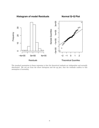
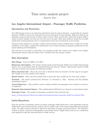
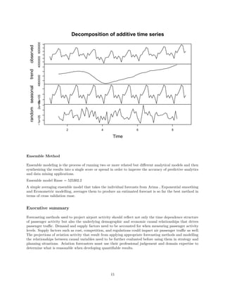
16. Forecasts from Holt−Winters' additive method
2 4 6 8 10
400000055000007000000
Time Series Decomposition
The decomposition of time series is a statistical method that deconstructs a time series into notional
components.
This is an important technique for all types of time series analysis, especially for seasonal adjustment. It
seeks to construct, from an observed time series, a number of component series (that could be used to
reconstruct the original by additions or multiplications) where each of these has a certain characteristic or
type of behaviour. For example, time series are usually decomposed into:
1. the Trend Component that reflects the long term progression of the series (secular variation)
2. the Cyclical Component that describes repeated but non-periodic fluctuations
3. the Seasonal Component reflecting seasonality (seasonal variation)
4. the Irregular Component (or “noise”) that describes random, irregular influences. It represents the
residuals of the time series after the other components have been removed.
Using the base R function for time series decomposition, we shall decompose the time series into seasonal,trend
and irregular components using the moving averages.
[source: wikipedia]
14

17. 40000006000000
observed
4800000
trend
−5e+05
seasonal
−1e+052e+05
2 4 6 8
random
Time
Decomposition of additive time series
Ensemble Method
Ensemble modeling is the process of running two or more related but different analytical models and then
synthesizing the results into a single score or spread in order to improve the accuracy of predictive analytics
and data mining applications.
Ensemble model Rmse = 525302.2
A simple averaging ensemble model that takes the individual forecasts from Arima , Exponential smoothing
and Econometric modelling, averages them to produce an entimated forecast is so far the best method in
terms of cross validation rmse.
Executive summary
Forecasting methods used to project airport activity should reflect not only the time dependence structure
of passenger activity but also the underlying demographic and economic causal relationships that drives
passenger traffic. Demand and supply factors need to be accounted for when measuring passenger activity
levels. Supply factors such as cost, competition, and regulations could impact air passenger traffic as well.
The projections of aviation activity that result from applying appropriate forecasting methods and modelling
the relationships between causal variables need to be further evaluated before using them in strategy and
planning situations. Aviation forecasters must use their professional judgement and domain expertise to
determine what is reasonable when developing quantifiable results.
15