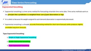
This document discusses time series analysis and forecasting using exponential smoothing methods. It provides textbooks and learning resources on time series analysis. It then describes the different types of exponential smoothing models - simple/single, double/Holt's trend, and triple/Holt-Winters. Examples are given showing how to implement these methods in Python using real-world airline passenger data and evaluate forecasts. Frequently asked questions are also included to summarize the key exponential smoothing techniques.

1. Time Series Analysis
TEXTBOOKS/LEARNING RESOURCES:
1. Aileen Nielsen, Practical Time Series Analysis: Prediction with Statistics and Machine Learning (1 ed.), O′Reilly, 2019. ISBN 1492041653.
2. Terence C. Mills, Applied Time Series Analysis: A Practical Guide to Modelling and Forecasting (1 ed.), Academic Press, 2019. ISBN 978-0-12-
813117-6.
REFERENCE BOOKS/LEARNING RESOURCES:
1. Aileen Nielsen, Practical Time Series Analysis: Prediction with Statistics and Machine Learning (1 ed.), O′Reilly, 2019. ISBN 1492041653.

2. 2
20 October 2023
Dr. Tej Bahadur Chandra
Time series Forecasting
Exponential Smoothing
Holt- Winters

3. 3
20 October 2023
Dr. Tej Bahadur Chandra
Time Series Forecasting
Exponential Smoothing
 Exponential smoothing is a time series method for forecasting univariate time series data. Time series methods work on
the principle that a prediction is a weighted linear sum of past observations or lags.
 It is called so because the weight assigned to each demand observation is exponentially decreased.
 Exponential smoothing is a broadly accurate forecasting method for short-term forecasts while produces slightly
unreliable long-term forecasts.
Types Exponential Smoothing:
1. Simple or Single Exponential Smoothing
2. Double Exponential Smoothing
3. Triple Exponential Smoothing

4. 4
20 October 2023
Dr. Tej Bahadur Chandra
Time Series Forecasting
Simple or Single Exponential Smoothing
 It is a time series forecasting method for univariate data without a trend or seasonality.
 It requires a single parameter, called alpha (between 0 and 1), also called the smoothing factor or smoothing
coefficient.
A value close to 1 indicates fast learning (that is, only the most recent values influence the forecasts),
whereas a value close to 0 indicates slow learning (past observations have a large influence on forecasts).
The SES formula is given by:
𝒔𝒕 = 𝜶𝒙𝒕 + 𝟏 – 𝜶 𝒔𝒕−𝟏
Where,
𝑠𝑡 = smoothed statistic (simple weighted average of current observation 𝑥𝑡)
𝑠𝑡−1 = previous smoothed statistic
α = smoothing factor of data; 0 < α < 1
t = time period

5. 5
20 October 2023
Dr. Tej Bahadur Chandra
Time Series Forecasting
Double Exponential Smoothing / Holt’s Trend Model
 It explicitly adds support for trends in the univariate time series. This method is known as Holt's trend model.
 In addition to the alpha(α) parameter, it needs another smoothing factor called beta (β), which controls the decay of
the influence of change in trend.
 Additive ways (smoothing with linear trend)
 Multiplicative ways (smoothing with exponential trend).
Beta (β) can be between 0 and 1. Higher values place more weight on recent observations, allowing the trend component
to react more quickly to changes in the trend.

6. 6
20 October 2023
Dr. Tej Bahadur Chandra
Time Series Forecasting
Triple Exponential Smoothing
 Triple Exponential Smoothing is an extension of Exponential Smoothing that explicitly adds support for seasonality to
the univariate time series.
 Also known as Holt-Winters Exponential Smoothing, named for two contributors to the method: Charles Holt and
Peter Winters.
In addition to the alpha and beta smoothing factors, a new parameter is added called gamma (g) that controls the
influence on the seasonal component.

7. 7
20 October 2023
Dr. Tej Bahadur Chandra
Example 1: Simple Exponential Smoothing
import pandas as pd
from statsmodels.tsa.api import SimpleExpSmoothing
import plotly.express as px
import matplotlib.pyplot as plt
from statsmodels.tsa.seasonal import seasonal_decompose
#Read the data
df=pd.read_csv('AirPassengers.csv')
df.Passengers=df.Passengers.diff(1) #Remove trend
df.Passengers=df.Passengers.diff(12) #Remove Seasonality
df=df.dropna()
df=df.reset_index(drop=True)
n=12 #define forecast period
alpha=0.2 #0.8
#First Instance
modal1 = SimpleExpSmoothing(df.Passengers).fit(smoothing_level=alpha,optimized=False)
forecast1 = modal1.forecast(n).rename('alpha=' + str(alpha))

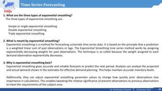
8. 8
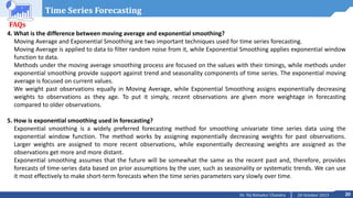
20 October 2023
Dr. Tej Bahadur Chandra
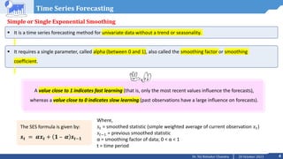
Example 1: Simple Exponential Smoothing
#Second Instance
modal3 = SimpleExpSmoothing(df.Passengers).fit()
forecast3 = modal3.forecast(n).rename('alpha=%s'%modal3.model.params['smoothing_level
'])
#After creating model we will visualize the plot
ax = df.plot(marker='o', color='black', figsize=(12,8), legend=True)
#Plot for alpha =0.2
forecast1.plot(marker='+', ax=ax, color='blue', legend=True)
modal1.fittedvalues.plot(marker='+', ax=ax, color='blue')
#Plot for alpha=Optimized by statsmodel
forecast3.plot(marker='*', ax=ax, color='green', legend=True)
modal3.fittedvalues.plot(marker='*', ax=ax, color='green')
plt.show()

9. 9
20 October 2023
Dr. Tej Bahadur Chandra
Example 1: Simple Exponential Smoothing

10. 10
20 October 2023
Dr. Tej Bahadur Chandra
Example 2: Double Exponential Smoothing / Holt’s Trend
import pandas as pd
from statsmodels.tsa.holtwinters import ExponentialSmoothing
import plotly.express as px
import matplotlib.pyplot as plt
from statsmodels.tsa.seasonal import seasonal_decompose
from sklearn.metrics import mean_squared_error
import numpy as np
#Read the data
df=pd.read_csv('AirPassengers.csv')
#df.Passengers=df.Passengers.diff(1) #Remove trend
df.Passengers=df.Passengers.diff(12) #Remove Seasonality
df=df.dropna()
df=df.reset_index(drop=True)
n=12 #define forecast period
alpha=0.2
trend='add'

11. 11
20 October 2023
Dr. Tej Bahadur Chandra
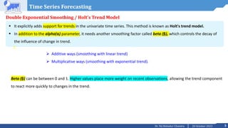
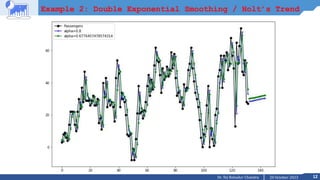
Example 2: Double Exponential Smoothing / Holt’s Trend
#First Instance
modal1 = ExponentialSmoothing(df.Passengers, trend).fit(smoothing_level=alpha)
forecast1 = modal1.forecast(n).rename('alpha='+str(alpha))
#Third Instance
modal3 = ExponentialSmoothing(df.Passengers, trend).fit()
forecast3 = modal3.forecast(n).rename('alpha=%s'%modal3.model.params['smoothing_level
'])
#After creating model we will visualize the plot
ax = df.plot(marker='o', color='black', figsize=(12,8), legend=True)
#Plot for alpha =0.2
forecast1.plot(marker='+', ax=ax, color='blue', legend=True)
modal1.fittedvalues.plot(marker='+', ax=ax, color='blue')
#Plot for alpha=Optimized by statsmodel
forecast3.plot(marker='*', ax=ax, color='green', legend=True)
modal3.fittedvalues.plot(marker='*', ax=ax, color='green')
plt.show()

12. 12
20 October 2023
Dr. Tej Bahadur Chandra
Example 2: Double Exponential Smoothing / Holt’s Trend

13. 13
20 October 2023
Dr. Tej Bahadur Chandra
Example 3: Triple Exponential Smoothing
import pandas as pd
from statsmodels.tsa.holtwinters import ExponentialSmoothing
import plotly.express as px
import matplotlib.pyplot as plt
from statsmodels.tsa.seasonal import seasonal_decompose
from sklearn.metrics import mean_squared_error
import numpy as np
#Read the data
df=pd.read_csv('AirPassengers.csv')
#df.Passengers=df.Passengers.diff(1) #Remove trend
#df.Passengers=df.Passengers.diff(12) #Remove Seasonality
n=48 #define forecast period
alpha=0.8
trend='add'
seasonal='mul'
sPeriod=12

14. 14
20 October 2023
Dr. Tej Bahadur Chandra
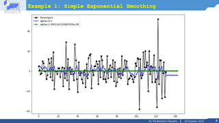
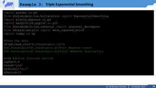
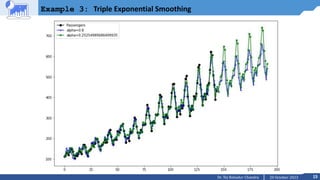
Example 3: Triple Exponential Smoothing
#First Instance
modal1 = ExponentialSmoothing(df.Passengers, trend, seasonal='add', seasonal_periods=sPer
iod).fit(smoothing_level=alpha)
forecast1 = modal1.forecast(n).rename('alpha='+str(alpha))
#Third Instance
modal3 = ExponentialSmoothing(df.Passengers, trend, seasonal='add', seasonal_periods=sPer
iod).fit()
forecast3 = modal3.forecast(n).rename('alpha=%s'%modal3.model.params['smoothing_level'])
#After creating model we will visualize the plot
ax = df.plot(marker='o', color='black', figsize=(12,8), legend=True)
#Plot for alpha =0.2
forecast1.plot(marker='+', ax=ax, color='blue', legend=True)
modal1.fittedvalues.plot(marker='+', ax=ax, color='blue')
#Plot for alpha=Optimized by statsmodel
forecast3.plot(marker='*', ax=ax, color='green', legend=True)
modal3.fittedvalues.plot(marker='*', ax=ax, color='green')
plt.show()

15. 15
20 October 2023
Dr. Tej Bahadur Chandra
Example 3: Triple Exponential Smoothing

16. 16
20 October 2023
Dr. Tej Bahadur Chandra
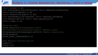
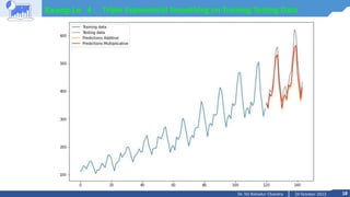
Example 4: Triple Exponential Smoothing on Training Testing Data
import pandas as pd
from statsmodels.tsa.holtwinters import ExponentialSmoothing
import plotly.express as px
import matplotlib.pyplot as plt
from statsmodels.tsa.seasonal import seasonal_decompose
from sklearn.metrics import mean_squared_error
import numpy as np
alpha=0.8
sPeriod=12
#Read the data
df=pd.read_csv('AirPassengers.csv')
df_train = df[:-24]
df_test = df[-24:]
# Additive model
model_add = ExponentialSmoothing(df_train['Passengers'], trend='add', seasonal='add',
seasonal_periods=sPeriod)
results_add = model_add.fit()
predictions_add = results_add.forecast(steps=24)

17. 17
20 October 2023
Dr. Tej Bahadur Chandra
Example 4: Triple Exponential Smoothing on Training Testing Data
# Multiplicative model
model_mul = ExponentialSmoothing(df_train['Passengers'], trend='mul', seasonal='add',
seasonal_periods=sPeriod)
results_mul = model_mul.fit()
predictions_mul = results_mul.forecast(steps=24)
# Evaluate
rmse_add = mean_squared_error(df_test['Passengers'], predictions_add, squared=False)
rmse_mul = mean_squared_error(df_test['Passengers'], predictions_mul, squared=False)
print('rmse_add = ', rmse_add)
print('rmse_mul = ', rmse_mul)
# Plot
plt.figure(figsize=(12,8))
plt.plot(df_train['Passengers'], label='Training data')
plt.plot(df_test['Passengers'], color='gray', label='Testing data')
plt.plot(predictions_add, color='orange', label='Predictions Additive')
plt.plot(predictions_mul, color='red', label='Predictions Multiplicative')
plt.legend();

18. 18
20 October 2023
Dr. Tej Bahadur Chandra
Example 4: Triple Exponential Smoothing on Training Testing Data

19. 19
20 October 2023
Dr. Tej Bahadur Chandra
Time Series Forecasting
FAQs
1. What are the three types of exponential smoothing?
The three types of exponential smoothing are:
Simple or single exponential smoothing
Double exponential smoothing
Triple exponential smoothing
2. What is meant by exponential smoothing?
Exponential smoothing is a method for forecasting univariate time series data. It is based on the principle that a prediction
is a weighted linear sum of past observations or lags. The Exponential Smoothing time series method works by assigning
exponentially decreasing weights for past observations. The technique is so called because the weight assigned to each
demand observation exponentially decreases.
3. Why is exponential smoothing best?
Exponential smoothing gives accurate and reliable forecasts to predict the next period. Analysts can analyze the projected
and actual demand shown in the estimates for effective demand planning. This helps maintain accurate inventory levels.
Additionally, they can adjust exponential smoothing parameter values to change how quickly prior observations lose
importance in calculations. This enables tweaking the relative significance of present observations to previous observations
to meet the requirements of the subject area.

20. 20
20 October 2023
Dr. Tej Bahadur Chandra
Time Series Forecasting
FAQs
4. What is the difference between moving average and exponential smoothing?
Moving Average and Exponential Smoothing are two important techniques used for time series forecasting.
Moving Average is applied to data to filter random noise from it, while Exponential Smoothing applies exponential window
function to data.
Methods under the moving average smoothing process are focused on the values with their timings, while methods under
exponential smoothing provide support against trend and seasonality components of time series. The exponential moving
average is focused on current values.
We weight past observations equally in Moving Average, while Exponential Smoothing assigns exponentially decreasing
weights to observations as they age. To put it simply, recent observations are given more weightage in forecasting
compared to older observations.
5. How is exponential smoothing used in forecasting?
Exponential smoothing is a widely preferred forecasting method for smoothing univariate time series data using the
exponential window function. The method works by assigning exponentially decreasing weights for past observations.
Larger weights are assigned to more recent observations, while exponentially decreasing weights are assigned as the
observations get more and more distant.
Exponential smoothing assumes that the future will be somewhat the same as the recent past and, therefore, provides
forecasts of time-series data based on prior assumptions by the user, such as seasonality or systematic trends. We can use
it most effectively to make short-term forecasts when the time series parameters vary slowly over time.

21. 21
20 October 2023
Dr. Tej Bahadur Chandra
Further Readings:
• https://machinelearningmastery.com/exponential-smoothing-for-time-series-forecasting-in-python/
• How to Select a Model For Your Time Series Prediction Task [Guide], https://neptune.ai/blog/select-model-for-time-series-
prediction-task